survalis
Interpretable Survival Machine Learning Framework
A modular toolkit for interpretable survival machine learning
with a unified interface for fitting, prediction, evaluation, and
interpretation.
It includes semiparametric, parametric, tree-based, ensemble, boosting,
kernel, and deep-learning survival learners, together with benchmarking,
scoring, calibration, and model-agnostic interpretation utilities.
Representative methodological anchors include Cox (1972)
survalis 
Unified survival machine learning and interpretability in R.


survalis provides a unified framework for survival machine learning in
R. Seven verbs cover the whole workflow for 22 built-in learners and for
any learner you write yourself: fitting, prediction, resampled and
external evaluation, tuning, paired comparison, model-agnostic
interpretation, and causal contrasts. Discrimination, calibration and
Brier metrics sit next to decision-weighted scores (dwscore()), which
average the loss of a risk-threshold decision rule over a stated range
of thresholds.
survalis is available on CRAN:
https://CRAN.R-project.org/package=survalis.
The seven-verb interface
library(survalis)
f <- Surv(time, status) ~ age + karno + celltype

m   <- fit(f, veteran, model = "ranger", spec = list(num.trees = 500))
predict(m, veteran[1:5, ], times = c(90, 180, 365))          # survival matrix
evaluate(m, times = c(90, 180, 365), resampling = cv(5))     # resampled metrics

cmp <- compare(f, veteran, models = c("coxph", "ranger", "densemlp"),
               times = c(90, 180, 365))
plot(cmp)

plot(interpret(m, "shap", newdata = veteran[1, ], times = 180))
estimate(f, veteran, model = "ranger", treatment = "trt", tau = 365)
fit(), predict(), evaluate(), tune(), compare(), interpret()
and estimate() are the whole interface. Resampling is described by
cv(), holdout(), groupcv() and bootstrap(), dwscore() scores a
survival matrix directly, and listlearners(), listmetrics() and
listmethods() give the valid ids. Upgrading from 1.x? See
vignette("from-1.0", package = "survalis").
Installation
# Install the released version from CRAN
install.packages("survalis")

# Or install the development version from GitHub
remotes::install_github("ielbadisy/survalis")
Core philosophy
- Seven verbs cover the whole workflow:
fit(),predict(),evaluate(),tune(),compare(),interpret(),estimate() - One function per job: learners are chosen by
model, metrics bymetrics, explanations bymethod, outputs bytype - Every verb returns an S3 object with
print(),summary(),plot()andas.data.frame()methods - Matrix predictions are survival matrices: one row per subject, columns
t=100,t=200, …, with the grid recorded inattr(x, "times") - A custom learner is two functions,
list(fit = , predict = ), and works with every verb
Exploring the package
library(survalis)
listlearners()               # ids for `model`
#>            learner tunable
#> 1            coxph   FALSE
#> 2            aalen   FALSE
#> 3           glmnet    TRUE
#> 4        selectcox    TRUE
#> 5           aftgee   FALSE
#> 6      flexsurvreg    TRUE
#> 7          bnnsurv    TRUE
#> 8            rpart    TRUE
#> 9             bart    TRUE
#> 10         xgboost    TRUE
#> 11        coxboost    TRUE
#> 12         fastgbm   FALSE
#> 13          ranger    TRUE
#> 14             rsf    TRUE
#> 15         cforest    TRUE
#> 16      blackboost    TRUE
#> 17         survsvm    TRUE
#> 18        densemlp   FALSE
#> 19            orsf    TRUE
#> 20          rpsurv   FALSE
#> 21          nbsurv   FALSE
#> 22 survmetalearner   FALSE
listmetrics()                    # ids for `metrics`
#>                  metric direction
#> 1                cindex  maximize
#> 2                   auc  maximize
#> 3                 brier  minimize
#> 4                   ibs  minimize
#> 5                   iae  minimize
#> 6                   ise  minimize
#> 7                   ece  minimize
#> 8               survacc  maximize
#> 9 range:<lower>-<upper>  minimize
#>                                                                                                        summary
#> 1                                                    Harrell-style concordance index for survival predictions.
#> 2                                         Cumulative/dynamic time-dependent AUC at a selected evaluation time.
#> 3                                     Brier Score at specified evaluation time(s) (IPCW-weighted when needed).
#> 4                                         Integrated Brier Score over an evaluation time grid (IPCW-weighted).
#> 5                                                    Integrated absolute error against the Kaplan-Meier curve.
#> 6                                                     Integrated squared error against the Kaplan-Meier curve.
#> 7                                                      Expected calibration error at a single evaluation time.
#> 8                           SurvAcc: spherical decision-weighted score at a single time (IPCW), see dwscore().
#> 9 Decision-weighted loss over a risk-threshold range, e.g. "range:0.05-0.20", at a single time, see dwscore().
#>                        range
#> 1  [0, 1] (higher is better)
#> 2  [0, 1] (higher is better)
#> 3   [0, 1] (lower is better)
#> 4   [0, 1] (lower is better)
#> 5 [0, Inf) (lower is better)
#> 6 [0, Inf) (lower is better)
#> 7   [0, 1] (lower is better)
#> 8  [0, 1] (higher is better)
#> 9   [0, 1] (lower is better)
listmethods()   # ids for `method` in interpret()
#>            method
#> 1             pdp
#> 2             ice
#> 3             ale
#> 4            shap
#> 5     shap_matrix
#> 6          varimp
#> 7         permute
#> 8     interaction
#> 9  counterfactual
#> 10      surrogate
#> 11 tree_surrogate
#> 12    calibration
#> 13            roc
#> 14            dca
#> 15    survcluster
#>                                                                    summary
#> 1      Partial dependence of predicted survival on one feature, over time.
#> 2               Individual conditional expectation curves for one feature.
#> 3                               Accumulated local effects for one feature.
#> 4                   Shapley values for one instance, aggregated over time.
#> 5                       Shapley values for many instances (beeswarm plot).
#> 6                   Permutation variable importance on the survival scale.
#> 7                                                         Alias of varimp.
#> 8                   Friedman H-statistic interaction strength per feature.
#> 9  Smallest feature changes that move predicted survival at a target time.
#> 10               Local linear surrogate for one instance at a target time.
#> 11                      Global decision-tree surrogate of the predictions.
#> 12                                          Calibration curve at one time.
#> 13                                   Time-dependent ROC curve at one time.
#> 14          Decision curve (net benefit over risk thresholds) at one time.
#> 15            Clusters of subjects with similar predicted survival curves.
Basic Workflow
1. Fit a model
mod_cox <- fit(Surv(time, status) ~ age + karno + celltype, veteran, model = "coxph")
mod_cox
#> <survalis_fit> model = coxph  (engine: survival)
#>   formula: Surv(time, status) ~ age + karno + celltype
#>   data:    137 obs, 128 events (93%)
2. Predict survival probabilities
pred <- predict(mod_cox, newdata = veteran[1:5, ], times = c(100, 200))
pred
#> <survmat> survival  |  5 obs x 2 times  [100, 200]
#>          t=100     t=200
#> [1,] 0.6142681 0.3541697
#> [2,] 0.6944383 0.4599242
#> [3,] 0.5556797 0.2860796
#> [4,] 0.6033305 0.3408724
#> [5,] 0.6959633 0.4620783
predict() also returns other quantities via type: "risk" (1 -
S(t)), "chf", "hazard", "rmst", "quantile", "median".
3. Evaluate model performance
ev <- evaluate(mod_cox, times = c(80, 160), resampling = cv(5, seed = 123))
ev
#> <survalis_eval> model = coxph
#> <survalis_resampling> 5-fold CV, strata = status, seed = 123
#>   grid: 2 times in [80, 160]
#>   cindex  0.7197  (sd 0.0532, 95% [0.6731, 0.7663], n = 5)
#>   ibs     0.1737  (sd 0.0379, 95% [0.1405, 0.2070], n = 5)
summary(ev)
#>   metric      mean         sd n         se     lower     upper
#> 1 cindex 0.7196779 0.05315293 5 0.02377071 0.6730873 0.7662685
#> 2    ibs 0.1737430 0.03790019 5 0.01694948 0.1405220 0.2069639
Metrics are chosen by metrics. Next to "cindex", "auc", "brier",
"ibs" and the calibration errors, the decision-weighted scores
"survacc" and "range:<lower>-<upper>" are available at a single
time.
To score a model on data it was not trained on, pass newdata; to score
predictions made elsewhere, pass the survival matrix and the outcome.
train <- veteran[1:100, ]
test  <- veteran[-(1:100), ]
m_tr  <- fit(Surv(time, status) ~ age + karno + celltype, train, model = "coxph")
evaluate(m_tr, newdata = test, times = c(80, 160))
#> <survalis_eval> model = coxph
#>   scored once on 37 subjects (no resampling)
#>   grid: 2 times in [80, 160]
#>   cindex  0.7485
#>   ibs     0.1424

S <- predict(m_tr, test, times = c(80, 160))
evaluate(S, y = Surv(test$time, test$status))
#> <survalis_eval> model = supplied predictions
#>   scored once on 37 subjects (no resampling)
#>   grid: 2 times in [80, 160]
#>   cindex  0.7485
#>   ibs     0.1424

evaluate(m_tr, newdata = test, times = 160,
         metrics = c("brier", "survacc", "range:0.05-0.20"))
#> <survalis_eval> model = coxph
#>   scored once on 37 subjects (no resampling)
#>   grid: 1 times in [160, 160]
#>   brier           0.0806
#>   survacc         0.9115
#>   range:0.05-0.20 0.0183
dwscore() gives the decision-weighted loss itself: the IPCW loss of
the rule “act if predicted risk exceeds c”, averaged over thresholds c
with a chosen weight ("range", "survacc", "brier", "log" or
"beta"). Each score is a weighted area under the net benefit curve.
y <- Surv(test$time, test$status)
dwscore(S, y, weight = "range", thresholds = c(0.05, 0.20))
#>   time          weight       loss
#> 1   80 range(0.05,0.2) 0.04391892
#> 2  160 range(0.05,0.2) 0.01829955
dwscore(S, y, weight = "survacc")
#>   time  weight       loss
#> 1   80 survacc 0.15888225
#> 2  160 survacc 0.08852427
4. Compare multiple learners
compare() evaluates every learner on the same resampling folds, so
results are paired; tune = TRUE tunes each tunable learner first.
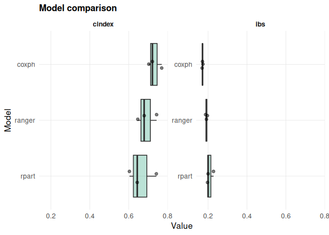
cmp <- compare(
  Surv(time, status) ~ age + karno + celltype,
  data = veteran,
  models = c("coxph", "rpart", "ranger"),
  times = c(80, 160),
  resampling = cv(3, seed = 1)
  )

cmp
#> <survalis_compare> 3 models
#> <survalis_resampling> 3-fold CV, strata = status, seed = 1
#>
#>   cindex (higher is better):
#>    * coxph            0.7317  (se 0.0199)
#>      ranger           0.6898  (se 0.0284)
#>      rpart            0.6634  (se 0.0411)
#>
#>   ibs (lower is better):
#>    * coxph            0.1713  (se 0.0012)
#>      ranger           0.1914  (se 0.0026)
#>      rpart            0.2085  (se 0.0099)
plot(cmp)
5. Tune a learner
tune() scores a grid of configurations on shared folds and refits the
best one. Learners with tunable = TRUE have a default grid; any
learner, custom ones included, can be tuned over a grid you supply.
tuned <- tune(
  Surv(time, status) ~ age + karno + celltype, veteran, model = "rpart",
  grid = expand.grid(cp = c(0.001, 0.01, 0.05), minsplit = c(10, 20), maxdepth = 5),
  times = c(80, 160), resampling = cv(3, seed = 1), metric = "ibs"
  )
tuned
#> <survalis_tune> model = rpart  |  optimise ibs over 6 configs
#> <survalis_resampling> 3-fold CV, strata = status, seed = 1
#>   best: minsplit = 10, cp = 0.05, maxdepth = 5
#>   ibs at best: 0.1758
predict(tuned, veteran[1:3, ], times = c(80, 160))
#> <survmat> survival  |  3 obs x 2 times  [80, 160]
#>           t=80     t=160
#> [1,] 0.8010013 0.5484333
#> [2,] 0.8010013 0.5484333
#> [3,] 0.8010013 0.5484333
6. Bring your own learner
A custom learner is a list with a fit function and a predict
function that returns one row per subject and one column per time. It
then works with every verb.
expo <- list(
  name = "exponential",
  fit = function(formula, data, ...) survival::survreg(formula, data, dist = "exponential"),
  predict = function(object, newdata, times) {
    rate <- 1 / predict(object, newdata, type = "response")
    exp(-outer(rate, times))
  }
)

compare(Surv(time, status) ~ age + karno + celltype, veteran,
        models = list("coxph", expo), times = c(80, 160),
        resampling = cv(3, seed = 1))
#> <survalis_compare> 2 models
#> <survalis_resampling> 3-fold CV, strata = status, seed = 1
#>
#>   cindex (higher is better):
#>    * exponential      0.7339  (se 0.0208)
#>      coxph            0.7317  (se 0.0199)
#>
#>   ibs (lower is better):
#>    * exponential      0.1712  (se 0.0031)
#>      coxph            0.1713  (se 0.0012)
7. Visualize interpretation
interpret() is the single entry point to every explanation method, and
plot() draws its result.
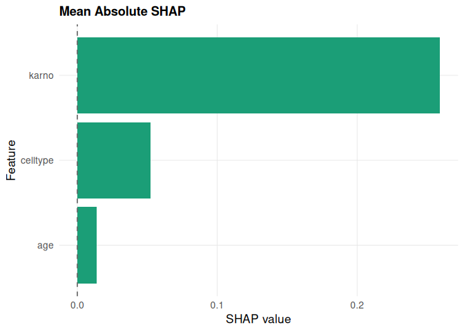
shap_meanabs <- interpret(
  mod_cox, "shap",
  newdata     = veteran[100, ],
  times       = 80,
  sample.size = 50,
  aggregate   = TRUE,
  shap_method = "meanabs"
  )

as.data.frame(shap_meanabs)
#>           feature        phi
#> age           age 0.01389376
#> karno       karno 0.25916597
#> celltype celltype 0.05208896
plot(shap_meanabs)
More interpretability methods
survalis also provides PDP, ALE, surrogate explanations, tree
surrogates, permutation importance, interaction analysis,
counterfactuals, and clustering of individualized survival curves, all
through interpret(fit, method = ..., ...).
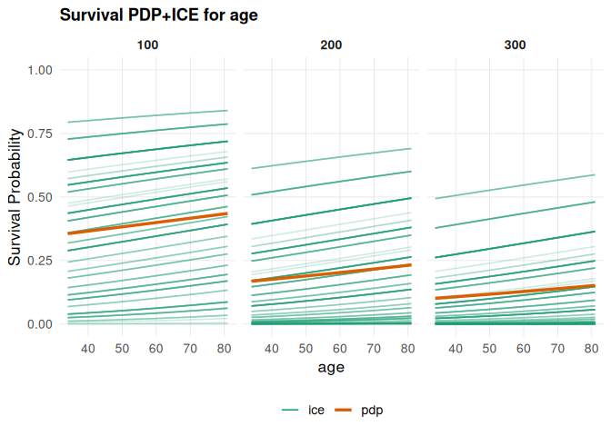
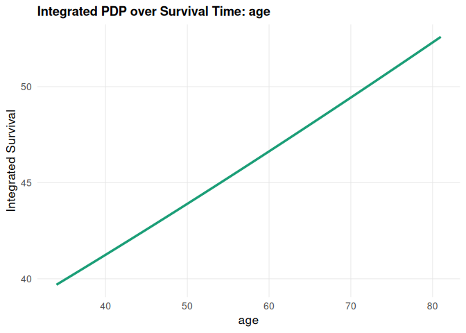
Partial dependence and ICE
pdp_age <- interpret(mod_cox, "pdp", feature = "age", times = c(100, 200, 300))

plot(pdp_age, which = "per_time")
plot(pdp_age, which = "integrated", smooth = TRUE)
#> `geom_smooth()` using formula = 'y ~ x'
Accumulated local effects
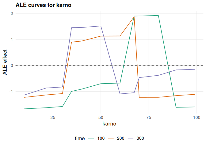
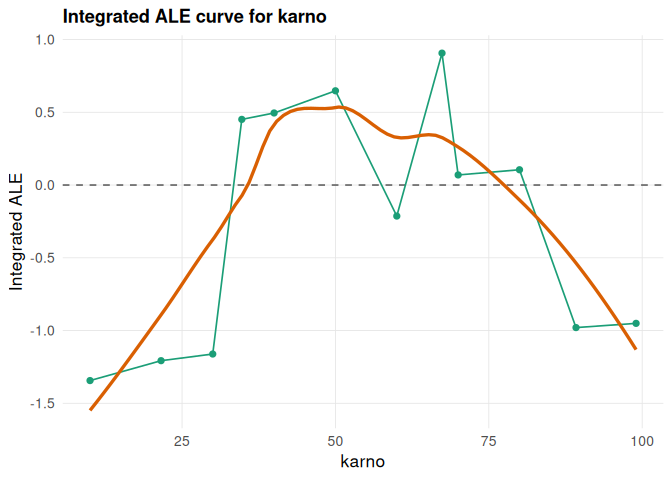
ale_karno <- interpret(mod_cox, "ale", feature = "karno", times = c(100, 200, 300))
#> Warning in rowsum(diffs, factor(bin, levels = seq_len(K)))/pmax(nk, 1L): longer
#> object length is not a multiple of shorter object length
#> Warning in matrix(apply(local, 2L, cumsum), nrow = K, ncol = n_times): data
#> length [27] is not a sub-multiple or multiple of the number of rows [11]

plot(ale_karno, which = "per_time")
plot(ale_karno, which = "integrated", smooth = TRUE)
#> `geom_smooth()` using formula = 'y ~ x'
Local surrogate explanation
local_surrogate <- interpret(
  mod_cox, "surrogate",
  newdata     = veteran[1, , drop = FALSE],
  times       = c(100, 200, 300),
  target_time = 200,
  k           = 5
  )
#> Warning in (function (model, newdata, baseline_data, times, target_time, :
#> Selected fewer variables than requested k.

as.data.frame(local_surrogate)
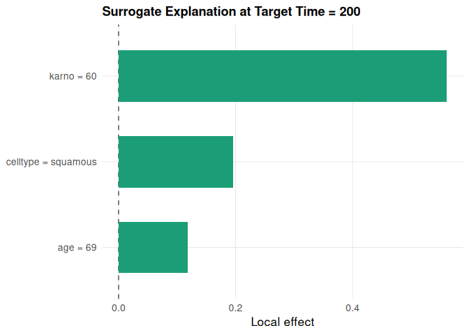
#>    feature feature_value    effect target_time
#> 1    karno            60 0.5605597         200
#> 2 celltype      squamous 0.1955526         200
#> 3      age            69 0.1184320         200
plot(local_surrogate, top_n = 10)
Tree surrogate
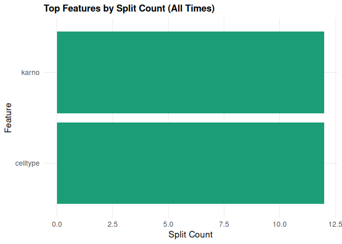
tree_surrogate <- interpret(mod_cox, "tree_surrogate", times = c(100, 200, 300))

plot(tree_surrogate, type = "importance", top_n = 5)
# plot(tree_surrogate, type = "tree")
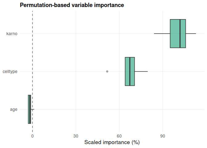
Permutation variable importance
varimp_res <- interpret(
  mod_cox, "varimp",
  times          = c(100, 200, 300),
  metric         = "ibs",
  n_repetitions  = 5,
  seed           = 123
  )

as.data.frame(varimp_res)
#>    feature    importance importance_05 importance_95 scaled_importance
#> 1    karno  0.0626237800   0.054011871  0.0698607609        100.000000
#> 2 celltype  0.0417312411   0.033900675  0.0487391810         66.638011
#> 3      age -0.0009593704  -0.001832599  0.0004581782         -1.531959
plot(varimp_res)
Feature interactions
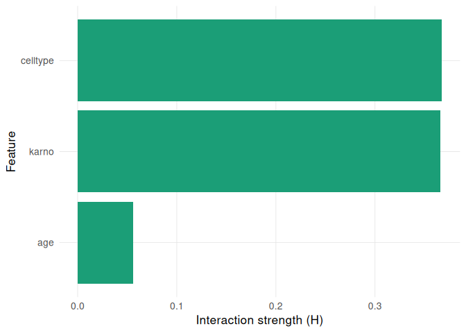
interaction_1way <- interpret(mod_cox, "interaction", times = c(100, 200, 300),
                              target_time = 200, type = "1way")
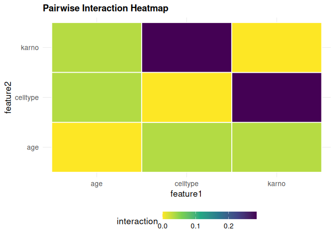
interaction_heatmap <- interpret(mod_cox, "interaction", times = c(100, 200, 300),
                                 target_time = 200, type = "heatmap")
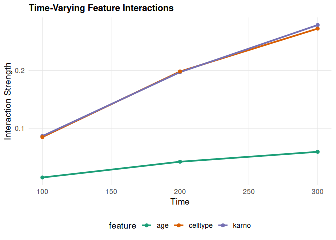
interaction_time <- interpret(mod_cox, "interaction", times = c(100, 200, 300),
                              type = "time")

plot(interaction_1way, type = "1way")
plot(interaction_heatmap, type = "heatmap")
plot(interaction_time, type = "time")
Counterfactual explanations
counterfactuals <- interpret(
  mod_cox, "counterfactual",
  newdata            = veteran[1, , drop = FALSE],
  times              = c(100, 200, 300),
  target_time        = 200,
  features_to_change = c("age", "karno", "diagtime"),
  cost_penalty       = 0.01
  )

as.data.frame(counterfactuals)
#>   feature original_value suggested_value survival_gain change_cost
#> 1     age             69         69.1313        0.0003      0.1313
#> 2   karno             60         81.0202        0.2347     21.0202
#>   penalized_gain
#> 1        -0.0010
#> 2         0.0245
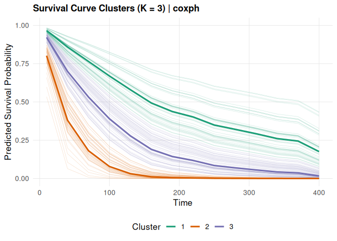
Clusters of survival curves
clusters <- interpret(mod_cox, "survcluster", times = seq(10, 400, by = 30),
                      K = 3, seed = 1)
plot(clusters)
8. Calibration, ROC and decision curves
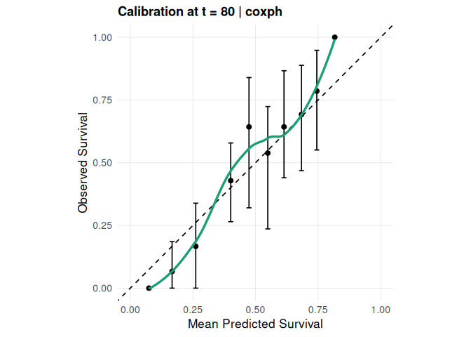
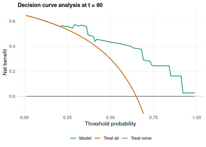
The decision curve uses the same censoring weights as dwscore(), so
each "range:<lower>-<upper>" loss equals the weighted area between the
treat-all and model curves.
interpret(mod_cox, "calibration", eval_time = 80, n_bins = 10, n_boot = 30) |> plot()
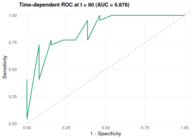
interpret(m_tr, "roc", newdata = test, eval_time = 80) |> plot()
interpret(m_tr, "dca", newdata = test, eval_time = 80) |> plot()
9. Causal contrasts
estimate() gives a plug-in G-formula contrast (RMST or survival,
difference or ratio) with bootstrap intervals. See
vignette("causal-estimation", package = "survalis").
estimate(Surv(time, status) ~ age + karno + celltype, veteran, model = "coxph",
         treatment = "trt", tau = 365, R = 50, seed = 1)
#> <survalis_estimate> RMST difference at tau = 365  (model: coxph)
#>   treatment: trt  (2 vs 1)
#>   estimate: -14.8805   95% CI [-46.7194, 11.2846]   (50 bootstrap, refit)
#>   plug-in G-formula; causal reading needs exchangeability, positivity,
#>   consistency, no interference and a correct outcome model.
Citation
citation("survalis")
#> To cite survalis in publications, use:
#>
#>   El Badisy I (2026). _survalis: Interpretable Survival Machine
#>   Learning Framework_. R package version 2.3.0,
#>   <https://CRAN.R-project.org/package=survalis>.
#>
#> A BibTeX entry for LaTeX users is
#>
#>   @Manual{,
#>     title = {survalis: Interpretable Survival Machine Learning Framework},
#>     author = {Imad {El Badisy}},
#>     year = {2026},
#>     note = {R package version 2.3.0},
#>     url = {https://CRAN.R-project.org/package=survalis},
#>   }