Convenient Functions for Exploratory Data Analysis

A collection of convenient functions to facilitate common tasks in exploratory data analysis. Some common tasks include generating summary tables of variables, displaying tables as a 'flextable' or a 'kable' and visualising variables using 'ggplot2'. Labels stating the source file with run time can be easily generated for annotation in tables and plots.

edar

The goal of edar is to provide some convenient functions to facilitate common tasks in exploratory data analysis.

Citation

Sou T (2025). edar: Convenient Functions for Exploratory Data Analysis. R package version 0.0.6, https://github.com/soutomas/edar.

Installation

# From CRAN - for the latest CRAN release 
install.packages("edar")

# From GitHub - for the development version
# install.packages("pak")
pak::pak("soutomas/edar")

Example

Summary

It is often helpful to see a quick summary of the dataset.

library(edar)
#> 
#> Attaching package: 'edar'
#> The following object is masked from 'package:stats':
#> 
#>     filter

# Data 
dat = mtcars |> mutate(across(c(am,carb,cyl,gear,vs),factor))

# Summaries of all continuous variables. 
dat |> summ_by()
#> NB: Non-numeric variables are dropped.
#> Dropped: cyl vs am gear carb
#> Adding missing grouping variables: `name`
#> # A tibble: 6 × 10
#>   name      n   nNA   Mean      SD   Min    P25    Med    P75    Max
#>   <chr> <int> <int>  <dbl>   <dbl> <dbl>  <dbl>  <dbl>  <dbl>  <dbl>
#> 1 disp     32     0 231.   124.    71.1  121.   196.   326    472   
#> 2 drat     32     0   3.60   0.535  2.76   3.08   3.70   3.92   4.93
#> 3 hp       32     0 147.    68.6   52     96.5  123    180    335   
#> 4 mpg      32     0  20.1    6.03  10.4   15.4   19.2   22.8   33.9 
#> 5 qsec     32     0  17.8    1.79  14.5   16.9   17.7   18.9   22.9 
#> 6 wt       32     0   3.22   0.978  1.51   2.58   3.32   3.61   5.42

# Summaries of a selected variable after grouping. 
dat |> summ_by(mpg,vs)
#> Adding missing grouping variables: `vs`
#> # A tibble: 2 × 10
#>   vs        n   nNA  Mean    SD   Min   P25   Med   P75   Max
#>   <fct> <int> <int> <dbl> <dbl> <dbl> <dbl> <dbl> <dbl> <dbl>
#> 1 0        18     0  16.6  3.86  10.4  14.8  15.6  19.1  26  
#> 2 1        14     0  24.6  5.38  17.8  21.4  22.8  29.6  33.9

# Summaries of all categorical variables. 
dat |> summ_cat()
#> NB: Numeric variables are dropped.
#> Dropped: mpg disp hp drat wt qsec
#> $cyl
#>    cyl  n percent
#>      4 11 0.34375
#>      6  7 0.21875
#>      8 14 0.43750
#>  Total 32 1.00000
#> 
#> $vs
#>     vs  n percent
#>      0 18  0.5625
#>      1 14  0.4375
#>  Total 32  1.0000
#> 
#> $am
#>     am  n percent
#>      0 19 0.59375
#>      1 13 0.40625
#>  Total 32 1.00000
#> 
#> $gear
#>   gear  n percent
#>      3 15 0.46875
#>      4 12 0.37500
#>      5  5 0.15625
#>  Total 32 1.00000
#> 
#> $carb
#>   carb  n percent
#>      1  7 0.21875
#>      2 10 0.31250
#>      3  3 0.09375
#>      4 10 0.31250
#>      6  1 0.03125
#>      8  1 0.03125
#>  Total 32 1.00000

Tables

Results can be viewed directly in a flextable object.

# Show data frame as a flextable object. 
dat |> summ_by(mpg,vs) |> ft()
#> Adding missing grouping variables: `vs`

Visualisation

Variables can be quickly visualised for exploratory graphical analysis.

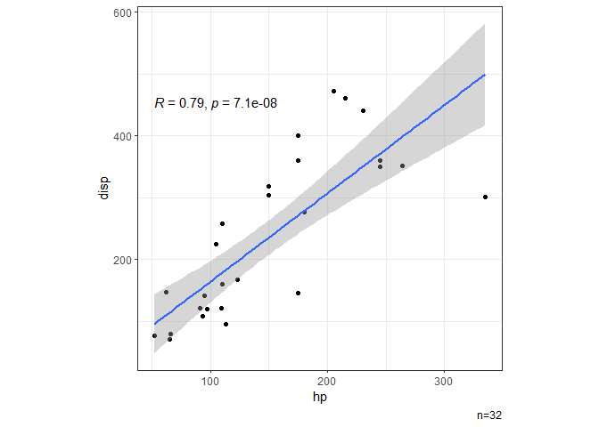
# Scatter plot showing correlation. 
dat |> ggxy(hp,disp)
#> `geom_smooth()` using formula = 'y ~ x'

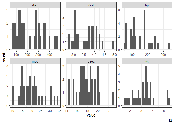
# Histograms of all continuous variables. 
dat |> gghist()
#> NB: Non-numeric variables are dropped.
#> Dropped: cyl vs am gear carb

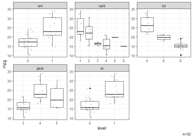
# Box plots stratified by categorical variables. 
dat |> ggbox(mpg)
#> NB: Numeric variables are dropped.
#> Dropped: disp hp drat wt qsec

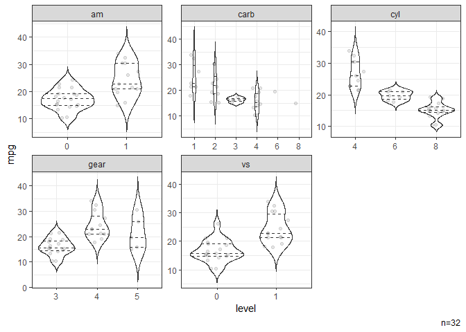
# Violin plots stratified by categorical variables. 
dat |> ggvio(mpg)
#> NB: Numeric variables are dropped.
#> Dropped: disp hp drat wt qsec
#> Warning: Groups with fewer than two datapoints have been dropped.
#> ℹ Set `drop = FALSE` to consider such groups for position adjustment purposes.
#> Groups with fewer than two datapoints have been dropped.
#> ℹ Set `drop = FALSE` to consider such groups for position adjustment purposes.

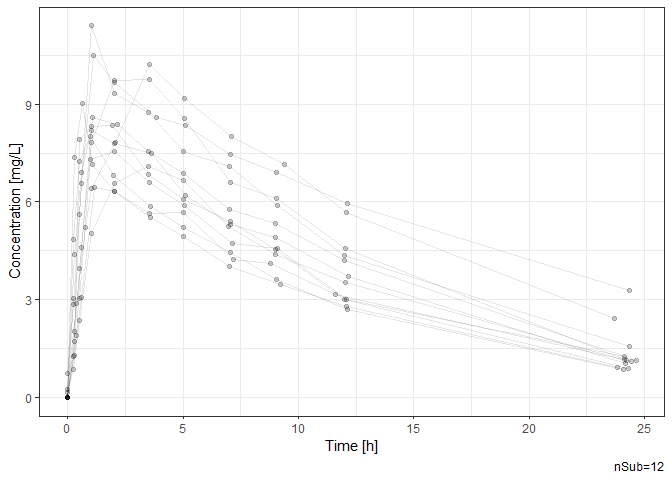
# Time-profile plot by subject.
Theoph |> ggtpp(Time, conc, id=Subject, xlab="Time [h]", ylab="Concentration [mg/L]")

Labels

A label indicating the current source file with a time stamp can be easily generated for annotation.

# To generate a source file label for annotation.
lab = label_src()

# A source file label can be directly added to the flextable output. 
dat |> summ_by(mpg,vs) |> ft(src=1)

# A source file label can be directly added to a ggplot object. 
p = dat |> ggxy(hp,disp)
p |> ggsrc()