rtables
Reporting Tables
Reporting tables often have structure that goes beyond simple rectangular data. The 'rtables' package provides a framework for declaring complex multi-level tabulations and then applying them to data. This framework models both tabulation and the resulting tables as hierarchical, tree-like objects which support sibling sub-tables, arbitrary splitting or grouping of data in row and column dimensions, cells containing multiple values, and the concept of contextual summary computations. A convenient pipe-able interface is provided for declaring table layouts and the corresponding computations, and then applying them to data.
rtables 


Reporting Tables with R
The rtables R package was designed to create and display complex
tables with R. The cells in an rtable may contain any high-dimensional
data structure which can then be displayed with cell-specific formatting
instructions. Currently, rtables can be outputted in ascii html,
and pdf, as well Power Point (via conversion to flextable objects).
rtf support is in development and will be in a future release.
rtables is developed and copy written by F. Hoffmann-La Roche and it
is released open source under Apache License Version 2.
rtables development is driven by the need to create regulatory ready
tables for health authority review. Some of the key requirements for
this undertaking are listed below:
- cell values and their visualization separate (i.e. no string based
tables)
- values need to be programmatically accessible in their non-rounded state for cross-checking
- multiple values displayed within a cell
- flexible tabulation framework
- flexible formatting (cell spans, rounding, alignment, etc.)
- multiple output formats (html, ascii, latex, pdf, xml)
- flexible pagination in both horizontal and vertical directions
- distinguish between name and label in the data structure to work with
CDISCstandards - title, footnotes, cell cell/row/column references
rtables currently covers virtually all of these requirements, and
further advances remain under active development.
Installation
rtables is available on CRAN and you can install the latest released
version with:
install.packages("rtables")
or you can install the latest development version directly from GitHub with:
# install.packages("pak")
pak::pak("pharmaverse/rtables")
Packaged releases (both those on CRAN and those between official CRAN releases) can be found in the releases list.
To understand how to use this package, please refer to the Introduction
to
rtables
article, which provides multiple examples of code implementation.
Cheatsheet
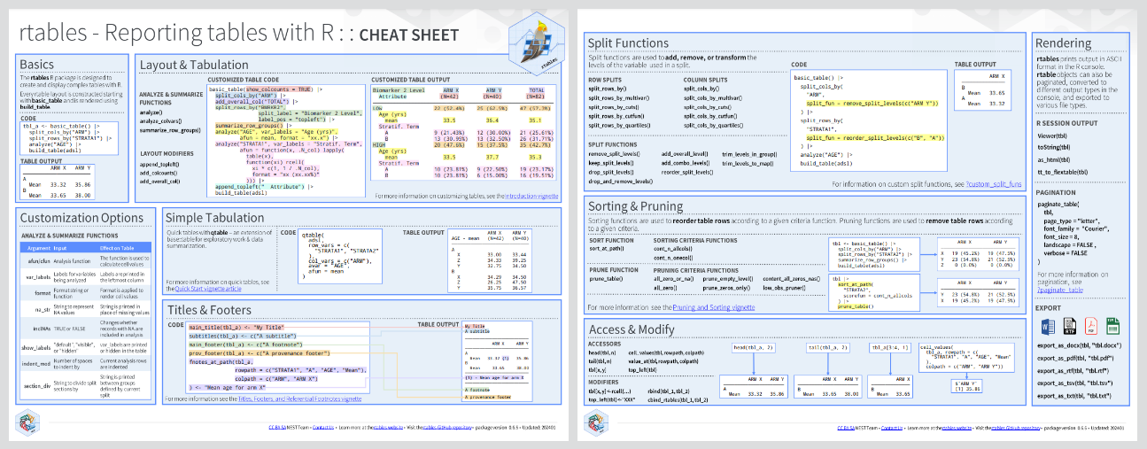
Usage
We first demonstrate with a demographic table-like example and then show the creation of a more complex table.
library(rtables)

lyt <- basic_table() |>
  split_cols_by("ARM") |>
  analyze(c("AGE", "BMRKR1", "BMRKR2"), function(x, ...) {
    if (is.numeric(x)) {
      in_rows(
        "Mean (sd)" = c(mean(x), sd(x)),
        "Median" = median(x),
        "Min - Max" = range(x),
        .formats = c("xx.xx (xx.xx)", "xx.xx", "xx.xx - xx.xx")
      )
    } else if (is.factor(x) || is.character(x)) {
      in_rows(.list = list_wrap_x(table)(x))
    } else {
      stop("type not supported")
    }
  })

build_table(lyt, ex_adsl)
#>                 A: Drug X      B: Placebo     C: Combination
#> ————————————————————————————————————————————————————————————
#> AGE
#>   Mean (sd)   33.77 (6.55)    35.43 (7.90)     35.43 (7.72)
#>   Median          33.00           35.00           35.00
#>   Min - Max   21.00 - 50.00   21.00 - 62.00   20.00 - 69.00
#> BMRKR1
#>   Mean (sd)    5.97 (3.55)     5.70 (3.31)     5.62 (3.49)
#>   Median          5.39            4.81             4.61
#>   Min - Max   0.41 - 17.67    0.65 - 14.24     0.17 - 21.39
#> BMRKR2
#>   LOW              50              45               40
#>   MEDIUM           37              56               42
#>   HIGH             47              33               50
library(rtables)
library(dplyr)

## for simplicity grab non-sparse subset
ADSL <- ex_adsl |> filter(RACE %in% levels(RACE)[1:3])

biomarker_ave <- function(x, ...) {
  val <- if (length(x) > 0) round(mean(x), 2) else "no data"
  in_rows(
    "Biomarker 1 (mean)" = rcell(val)
  )
}

basic_table(show_colcounts = TRUE) |>
  split_cols_by("ARM") |>
  split_cols_by("BMRKR2") |>
  split_rows_by("RACE", split_fun = trim_levels_in_group("SEX")) |>
  split_rows_by("SEX") |>
  summarize_row_groups() |>
  analyze("BMRKR1", biomarker_ave) |>
  build_table(ADSL)
#>                                          A: Drug X                            B: Placebo                           C: Combination
#>                                LOW        MEDIUM        HIGH         LOW         MEDIUM       HIGH         LOW         MEDIUM        HIGH
#>                               (N=45)      (N=35)       (N=46)       (N=42)       (N=48)      (N=31)       (N=40)       (N=39)       (N=47)
#> ————————————————————————————————————————————————————————————————————————————————————————————————————————————————————————————————————————————
#> ASIAN
#>   F                         13 (28.9%)   9 (25.7%)   19 (41.3%)   9 (21.4%)    18 (37.5%)   9 (29.0%)   13 (32.5%)   9 (23.1%)    17 (36.2%)
#>     Biomarker 1 (mean)         5.23        6.17         5.38         5.64         5.55        4.33         5.46         5.48         5.19
#>   M                         8 (17.8%)    7 (20.0%)   10 (21.7%)   12 (28.6%)   10 (20.8%)   8 (25.8%)   5 (12.5%)    11 (28.2%)   16 (34.0%)
#>     Biomarker 1 (mean)         6.77        6.06         5.54         4.9          4.98        6.81         6.53         5.47         4.98
#>   U                          1 (2.2%)    1 (2.9%)     0 (0.0%)     0 (0.0%)     0 (0.0%)    1 (3.2%)     0 (0.0%)     1 (2.6%)     1 (2.1%)
#>     Biomarker 1 (mean)         4.68         7.7       no data      no data      no data       6.97       no data       11.93         9.01
#> BLACK OR AFRICAN AMERICAN
#>   F                         6 (13.3%)    3 (8.6%)    9 (19.6%)    6 (14.3%)    8 (16.7%)    2 (6.5%)    7 (17.5%)    4 (10.3%)     3 (6.4%)
#>     Biomarker 1 (mean)         5.01         7.2         6.79         6.15         5.26        8.57         5.72         5.76         4.58
#>   M                         5 (11.1%)    5 (14.3%)    2 (4.3%)     3 (7.1%)    5 (10.4%)    4 (12.9%)   4 (10.0%)    5 (12.8%)    5 (10.6%)
#>     Biomarker 1 (mean)         6.92        5.82        11.66         4.46         6.14        8.47         6.16         5.25         4.83
#>   U                          0 (0.0%)    0 (0.0%)     0 (0.0%)     0 (0.0%)     0 (0.0%)    0 (0.0%)     1 (2.5%)     1 (2.6%)     0 (0.0%)
#>     Biomarker 1 (mean)       no data      no data     no data      no data      no data      no data       2.79         9.82       no data
#>   UNDIFFERENTIATED           1 (2.2%)    0 (0.0%)     0 (0.0%)     0 (0.0%)     0 (0.0%)    0 (0.0%)     2 (5.0%)     0 (0.0%)     0 (0.0%)
#>     Biomarker 1 (mean)         9.48       no data     no data      no data      no data      no data       6.46       no data      no data
#> WHITE
#>   F                         6 (13.3%)    7 (20.0%)    4 (8.7%)    5 (11.9%)    6 (12.5%)    6 (19.4%)   6 (15.0%)     3 (7.7%)     2 (4.3%)
#>     Biomarker 1 (mean)         4.43        7.83         4.52         6.42         5.07        7.83         6.71         5.87         10.7
#>   M                          4 (8.9%)    3 (8.6%)     2 (4.3%)    6 (14.3%)     1 (2.1%)    1 (3.2%)     2 (5.0%)    5 (12.8%)     3 (6.4%)
#>     Biomarker 1 (mean)         5.81        7.23         1.39         4.72         4.58        12.87        2.3          5.1          5.98
#>   U                          1 (2.2%)    0 (0.0%)     0 (0.0%)     1 (2.4%)     0 (0.0%)    0 (0.0%)     0 (0.0%)     0 (0.0%)     0 (0.0%)
#>     Biomarker 1 (mean)         3.94       no data     no data        3.77       no data      no data     no data      no data      no data
Acknowledgments
We would like to thank everyone who has made rtables a better project
by providing feedback and improving examples & vignettes. The following
list of contributors is alphabetical:
Maximo Carreras, Francois Collins, Saibah Chohan, Tadeusz Lewandowski, Nick Paszty, Nina Qi, Jana Stoilova, Heng Wang, Godwin Yung
Presentations
- R in Pharma 2023
- R Medicine Virtual Conference 2023 [Video]
- Advanced rtables Training 2023 [Part 1 Slides] [Part 2 Slides]
- R in Pharma 2022 - Creating Submission-Quality Clinical Trial Reporting Tables in R with rtables [Slides] [Video]
- R Consortium 2022
- useR! 2020 - rtables Layouting and Tabulation Framework [Video]