Spatial and Environmental Blocking for Cross-Validation

Creates spatially or environmentally separated, or group-preserving, training and testing folds for k-fold, leave-group-out, and leave-one-out cross-validation. Provides spatial blocking, clustering, buffering, and nearest-neighbour distance-matching methods, together with tools to visualise folds, summarise fold sizes and class balance, and assess train–test separation and environmental novelty. Also estimates spatial autocorrelation ranges in point samples and continuous raster covariates to provide an initial distance scale for designing spatial folds. Methods are described in Valavi, R. et al. (2019) .

blockCV

Spatially and environmentally separated folds for cross-validation

The blockCV package creates spatially or environmentally separated training and testing folds for k-fold, leave-group-out, and leave-one-out (LOO) cross-validation. These folds support more realistic evaluation of models fitted to spatially structured data, including remote-sensing classification, soil mapping, and species distribution modelling.

Alongside several fold-construction strategies, blockCV provides tools for checking fold balance, comparing fold separation with the prediction domain, and identifying environmental extrapolation. It can also estimate spatial autocorrelation ranges in point data or continuous raster covariates, providing an initial distance scale to investigate when designing spatial folds.

Main features

Six fold-construction strategies: spatial blocks (cv_spatial), spatial or environmental clustering (cv_cluster), existing grouping factors (cv_group), buffering (cv_buffer), leave-one-out nearest neighbour distance matching (cv_nndm), and k-fold nearest neighbour distance matching (cv_knndm)
Hexagonal (default), rectangular, or user-defined spatial blocks, assigned to folds using random, systematic, checkerboard, or predefined selection. Random assignment can search for balanced folds
Environmental clustering with optional spatial constraints through spatial_weight, and optional over-clustering to improve fold balance
Geographical or feature-space kNNDM using prediction locations supplied by a raster (r), prediction points (pred_points), or a polygon (model_domain), with block, hierarchical, or k-means grouping
Response-aware fold summaries and, where supported, balancing for binary, multi-class, continuous, count, and presence-background data. Continuous and count responses can be grouped into quantile bins using num_bins
Fold diagnostics through cv_summary, cv_distance, and cv_similarity to assess balance, train-test separation, agreement with prediction-domain distances, and environmental extrapolation
Fold visualisation with cv_plot, including faceted train-test maps for every strategy and combined-fold maps for k-fold methods
Spatial autocorrelation and interactive block-size tools (cv_spatial_autocor and cv_block_size) for exploring an initial separation distance
Raster processing with terra, including support for stars, raster, and raster files on disk

What's new in v4.0

Added cv_knndm for k-fold nearest neighbour distance matching, with geographical and feature-space matching and block, hierarchical, or k-means grouping
Added cv_group for leave-group-out cross-validation based on an existing site, plot, campaign, individual, or other grouping factor
Added cv_summary for one-call fold-quality summaries and warnings, and cv_distance for comparing fold separation with nearest-neighbour distances in the prediction domain
Expanded cv_similarity with per-fold extrapolation summaries, overall novelty rates, and spatial map visualisation
Made fold balancing explicit in cv_spatial, cv_cluster, and cv_knndm; added presence-background balancing and quantile binning (num_bins) for continuous or count responses
Added spatially-constrained environmental clustering through cv_cluster(spatial_weight = ...)
Added combined-fold maps to cv_plot and informative print methods for fold and diagnostic objects
Expanded cv_nndm and cv_knndm to accept prediction rasters, prediction points, or model-domain polygons
Removed the legacy v2.x function names. Other breaking changes include the new structured return value from cv_similarity, the rename of num_plot to num_plots, and interactive-only defaults for several automatic plots, reports, and progress bars

See NEWS.md for the full changelog.

Installation

To install the latest update of the package from GitHub use:

remotes::install_github("rvalavi/blockCV", build_vignettes = TRUE, dependencies = TRUE)

Or installing from CRAN:

install.packages("blockCV", dependencies = TRUE)

Vignettes

The package ships with several tutorials as vignettes:

blockCV introduction: how to create block cross-validation folds (tutorial_1)
Choosing and diagnosing spatial folds (tutorial_2)
Block cross-validation for species distribution modelling (tutorial_3)
Using blockCV with caret (tutorial_4)

To read them, install the package with the vignettes built (see Installation and use build_vignettes = TRUE), then open them from R:

# list all tutorials
browseVignettes("blockCV")

# or open one directly
vignette("tutorial_1", package = "blockCV")

Basic usage

The examples below highlight a few common workflows. See the vignettes for more information and complete examples.

# loading the package
library(blockCV)
library(sf) # working with spatial vector data
library(terra) # working with spatial raster data

# load raster data; the pipe operator |> is available in R v4.1 or higher
covars <- system.file("extdata/au/", package = "blockCV") |>
  list.files(full.names = TRUE) |>
  terra::rast()

# load species presence-absence data and convert to sf
pa_data <- read.csv(system.file("extdata/", "species.csv", package = "blockCV")) |>
  sf::st_as_sf(coords = c("x", "y"), crs = 7845)

# spatial blocking by specified range and random assignment
sb <- cv_spatial(
    x = pa_data,          # sf object of sample points (e.g. species data)
    column = "occ",       # optional response column for fold records/balancing
    r = covars,           # a raster for background (optional)
    size = 350000,        # size of the blocks in metres
    k = 5,                # number of folds
    hexagon = TRUE,       # use hexagonal blocks - default
    selection = "random", # random blocks-to-fold
    balance = TRUE,       # find balanced folds
    iteration = 100,      # search for balanced folds
    biomod2 = TRUE        # also create folds for biomod2
)

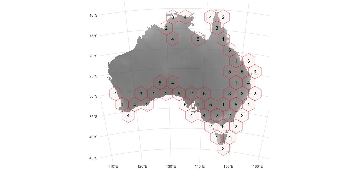
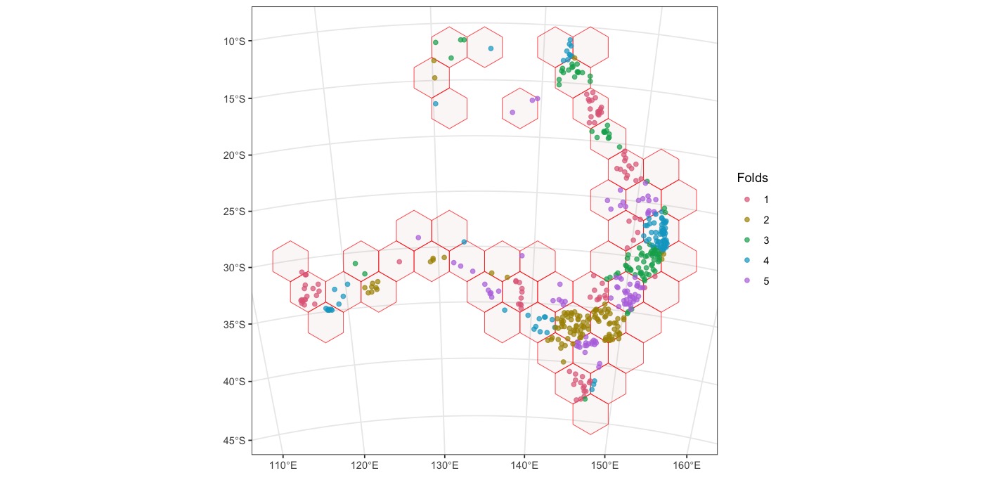
Use cv_plot() or the generic plot() method to visualise the folds.

plot(sb, pa_data, combine_folds = TRUE)

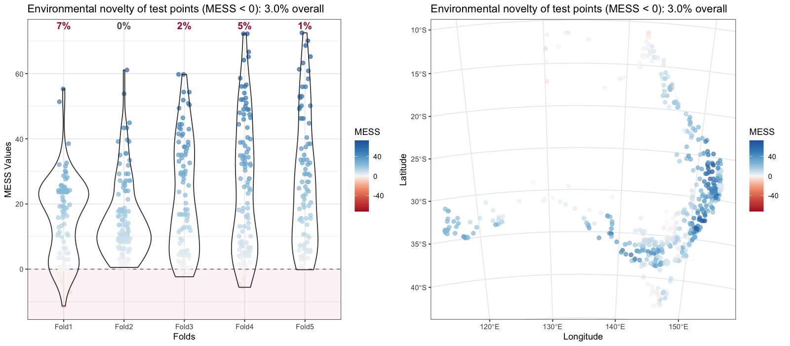
cv_similarity() compares each testing fold with its corresponding training data to identify environmental extrapolation. Negative MESS values flag test points outside the environmental range represented by their training data. The distribution and map views show how much extrapolation occurs and where, while the returned object also provides per-fold and overall summaries.

sim1 <- cv_similarity(cv = sb, x = pa_data, r = covars, method = "MESS")
sim2 <- cv_similarity(cv = sb, x = pa_data, r = covars, method = "MESS", type = "map")

sim_map <- sim2$plot +
    ggplot2::labs(x = "Longitude", y = "Latitude")

cowplot::plot_grid(sim1$plot, sim_map, nrow = 1)

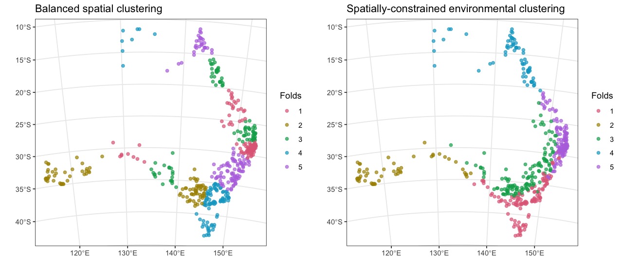
cv_cluster() can be tailored to different validation goals. For spatial clustering, balance = TRUE forms additional candidate clusters and assigns them to folds to improve record or response-class balance; k_multiplier controls the trade-off with geographical compactness. For environmental clustering, spatial_weight adds a soft geographical constraint so environmentally similar folds are less spatially scattered.

# balanced spatial clustering
set.seed(6)
bc <- cv_cluster(
    x = pa_data,
    column = "occ",
    k = 5,
    balance = TRUE,
    k_multiplier = 3
)

# spatially-constrained environmental clustering
set.seed(6)
sec <- cv_cluster(
    x = pa_data,
    r = covars,
    column = "occ",
    k = 5,
    spatial_weight = 0.4
)

bc_plot <- cv_plot(bc, x = pa_data, combine_folds = TRUE) +
    ggplot2::labs(title = "Balanced spatial clustering")

sec_plot <- cv_plot(sec, x = pa_data, combine_folds = TRUE) +
    ggplot2::labs(title = "Spatially-constrained environmental clustering")

cowplot::plot_grid(bc_plot, sec_plot, nrow = 1)

Create k-fold NNDM folds:

# k-fold nearest neighbour distance matching
knn <- cv_knndm(
    x = pa_data,
    column = "occ", # optionally prefer class-complete folds
    r = covars, # prediction area, or use pred_points/model_domain
    k = 5,
    num_sample = 5000
)

# compare an existing fold design with prediction-domain distances
cv_distance(
    cv = sb,
    x = pa_data,
    r = covars,
    num_sample = 5000
)

Investigate spatial autocorrelation in the landscape to choose a suitable size for spatial blocks:

# exploring the effective range of spatial autocorrelation in raster covariates or sample data
cv_spatial_autocor(
    r = covars, # a SpatRaster object or path to files
    num_sample = 5000, # number of cells to be used
    plot = TRUE
)

For the residual-based block-size guidance in Roberts et al. (2017), fit the model first, add its residuals to the sample points, and pass that residual column to cv_spatial_autocor(x = ..., column = ...). Ranges estimated from the raw response or raster covariates are exploratory proxies and may mis-size blocks for residual autocorrelation.

Alternatively, you can manually choose the size of spatial blocks in an interactive session using a Shiny app.

# a shiny interactive app to aid selecting a size for spatial blocks
cv_block_size(
    r = covars[[1]],
    x = pa_data, # optionally add sample points
    column = "occ",
    min_size = 2e5,
    max_size = 9e5
)

Reporting issues

Please report issues at: https://github.com/rvalavi/blockCV/issues

Acknowledgements

Special thanks to Eleanor Stern, who created the original artwork for the blockCV logo.

Citation

To cite package blockCV in publications, please use:

Valavi R, Elith J, Lahoz-Monfort JJ, Guillera-Arroita G. blockCV: An R package for generating spatially or environmentally separated folds for k-fold cross-validation of species distribution models. Methods Ecol Evol. 2019; 10:225--232. https://doi.org/10.1111/2041-210X.13107