Proximum
Statistical Analysis of Ensemble Proximity Matrices
Treats the proximity matrices produced by tree ensembles as first-class statistical objects rather than as model by-products. Provides a unified extractor across ensemble engines, in-bag and out-of-bag definitions, transformations to dissimilarities with metric diagnostics, corrections that make an indefinite proximity usable as a kernel, and permutation inference for comparing two proximity matrices or partitioning one across the terms of a design. Also provides a Nystrom approximation, a thresholded sparse representation and a streaming form that never allocates the matrix at all, for samples too large to hold it, measures how far the proximity moves between replicates of the ensemble, and draws each object through 'ggplot2': the seriated matrix, the configuration it implies, and the thresholded graph with its communities.
Proximum





Statistical analysis of the proximity matrices that tree ensembles produce.
The problem
Fit a random forest and you get predictions, and you get an importance table. You also get, whether you ask for it or not, an answer to a different question: which observations does this model consider to be the same kind of thing? Two observations that keep landing in the same leaf are, as far as the forest is concerned, alike. Collect that over every tree and you have the proximity matrix
$$P_{ij} = \frac{1}{B}\sum_{b=1}^{B} \mathbb{I}\big[\ell_b(x_i) = \ell_b(x_j)\big],$$
with $\ell_b(x)$ the leaf of tree $b$ that $x$ reaches. It is a full description of the geometry the model learned, and it is the only part of a forest that talks about the observations rather than about the variables.
randomForest will compute it if you pass proximity = TRUE, hand you
the matrix, and stop. There is no way in R to ask of it any of the
questions that make it a statistical object rather than a picture:
- Do two forests represent the data the same way? Two engines, two random seeds, this year's model against last year's.
- How much of the structure is explained by the response, and how much by something the model never saw?
- Is it stable? A matrix that changes when you refit is not evidence of anything, and nobody says how many trees it takes.
- What do you do when $n$ is large? The matrix is $n \times n$: 31 MB at $n = 2{,}000$ and about 760 MB at $n = 10{,}000$.
- Is it even a valid kernel? The out-of-bag definition, which is the one that removes the optimistic bias, is not positive semi-definite, and every method downstream that assumes a kernel is quietly wrong on it.
What the package does instead
One extractor across engines, both definitions, the transforms and
metric diagnostics that go with them, permutation inference for
comparing matrices and partitioning one, two storage forms for when the
matrix does not fit, a stability layer, and five plots. Every number in
the documentation comes from a simulation study shipped in
inst/simulations/, and several of those studies exist because they
contradicted something that had been written down first.
Installation
# install.packages("pak")
pak::pak("agostinognasso/Proximum")
A worked example, end to end
The package ships a synthetic consumer loan portfolio. It is generated
rather than collected, and ?loans says exactly what was built into it
and why; the short version is that public credit panels with a protected
attribute left in them do not exist, and one of the questions below
needs one.
library(Proximum)
library(randomForest)
#> randomForest 4.7-1.2
#> Type rfNews() to see new features/changes/bug fixes.

str(loans, give.attr = FALSE, vec.len = 2)
#> 'data.frame':    2000 obs. of  13 variables:
#>  $ default        : Factor w/ 2 levels "no","yes": 1 1 1 1 1 ...
#>  $ amount         : num  8125 4425 ...
#>  $ income         : num  27233 30134 ...
#>  $ dti            : num  0.436 0.255 0.385 0.562 0.397 ...
#>  $ term           : Factor w/ 2 levels "36 months","60 months": 2 1 2 1 1 ...
#>  $ employment     : num  6 7 17 0 3 ...
#>  $ score          : num  720 673 644 758 553 ...
#>  $ utilisation    : num  0.352 0.445 0.566 0.345 0.367 ...
#>  $ delinquencies  : int  0 2 0 0 0 ...
#>  $ home           : Factor w/ 3 levels "rent","mortgage",..: 3 3 2 2 2 ...
#>  $ purpose        : Factor w/ 5 levels "debt consolidation",..: 5 1 1 1 1 ...
#>  $ vintage        : Factor w/ 4 levels "2019","2020",..: 1 1 1 1 1 ...
#>  $ applicant_group: Factor w/ 2 levels "A","B": 1 1 1 1 2 ...
The proximity, and what it is
as_proximity() takes a fitted ensemble and the data it was fitted on.
predictors <- setdiff(names(loans), c("applicant_group", "vintage"))

set.seed(1)
book <- loans[sample(nrow(loans), 400), ]
rf <- randomForest(default ~ ., data = book[, predictors], ntree = 500)

px <- as_proximity(rf, newdata = book[, predictors])
px
#> <proximity> 400 x 400
#>   engine : randomForest
#>   trees  : 500
#>   type   : inbag
The name is as_proximity() and not proximity() because e2tree, the
package most likely to be attached alongside this one, exports a
proximity() of its own. The as_ prefix also says what it does: it
coerces a fitted ensemble into an object of class proximity, the way
as.dist() coerces into a dist.
summary() reports what the matrix looks like and, more usefully,
whether the dissimilarity it induces can be embedded in a Euclidean
space at all.
summary(px)
#> <proximity> summary
#>   observations : 400
#>   engine       : randomForest ( 500 trees )
#>   type         : inbag
#>   off-diagonal :
#>    0%   25%   50%   75%  100%
#> 0.000 0.010 0.052 0.156 0.972
#>   exact zeros  : 10.7%
#>   euclidean    : TRUE
The one thing everybody gets wrong
The in-bag proximity above averages over all trees, including the trees that were fitted on $i$ and $j$. Those trees have seen both observations and are inclined to separate them correctly, which inflates the proximity of same-class pairs. Restricting the average to the trees where both were out-of-bag removes that bias, and costs the geometry:
rf_oob <- randomForest(default ~ ., data = book[, predictors], ntree = 500,
                       keep.inbag = TRUE)
px_oob <- as_proximity(rf_oob, newdata = book[, predictors], type = "oob")

c(inbag = summary(px)$euclidean, oob = summary(px_oob)$euclidean)
#> inbag   oob
#>  TRUE FALSE
This is not an accident of the data. Stack the leaf indicators into $Z$:
the in-bag proximity is $P = ZZ^{\top}/B$, a Gram matrix, hence positive
semi-definite. The out-of-bag one divides each entry by the number of
trees in which that pair was jointly out of bag, making it a Hadamard
quotient of two Gram matrices, which need not be positive semi-definite
and here is not. Debiasing the estimate costs the geometry. make_psd()
will repair it and record what it did, and summary() refuses to let
the question pass silently either way.
Looking at it
Three views of the same object, and which one answers a question depends on the question.
autoplot(px, type = "heatmap")
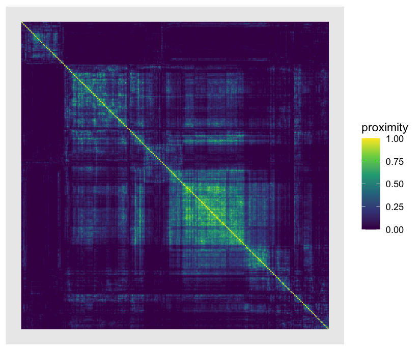
The rows and columns are ordered by a seriation of the induced dissimilarity, so the blocks the ensemble learned line up along the diagonal instead of being scattered by the order the rows arrived in.
autoplot(px, type = "mds", colour = book$default)
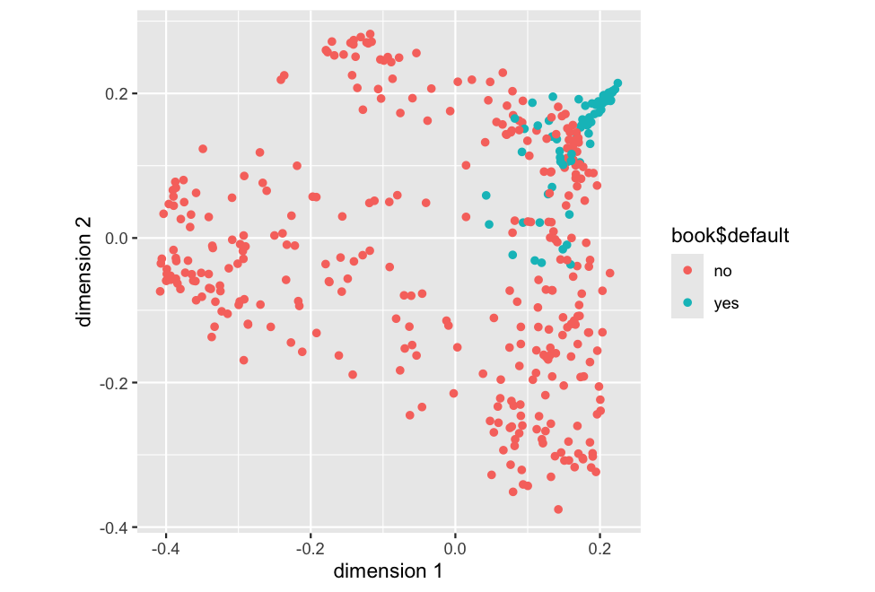
The colouring is yours to pass. A proximity object carries the engine,
the number of trees and the definition used, and nothing about the
response, so a plot that coloured by outcome on its own would be
inventing the outcome.
set.seed(11)
autoplot(px, type = "network", threshold = 0.2)
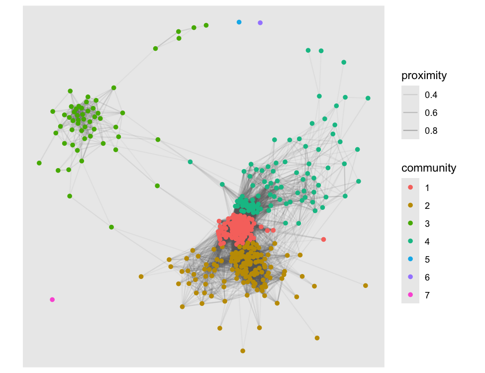
The network keeps the pairs above a threshold and reads the communities
of the graph that remain. Those communities are the forest's own
clustering, recovered from the proximity rather than imposed from
outside; vignette("credit-scoring-case") asks whether they are risk
segments and finds one that defaults at close to nine in ten against a
book rate of one in six.
Comparing two forests
This is the question the package was written for. Fit a second forest, on the same data, differing only in the seed, and ask whether the two represent the borrowers the same way.
rf2 <- randomForest(default ~ ., data = book[, predictors], ntree = 500)
px2 <- as_proximity(rf2, newdata = book[, predictors])

mantel_test(px, px2, n_perm = 999)
#>
#>  Mantel test (pearson, 999 permutations of the observations)
#>
#> data:  px and px2
#> r = 0.99192, pairs = 79800, permutations = 999, p-value = 0.001
#> alternative hypothesis: greater
Two refits of the same forest agree almost perfectly, which is the answer you would hope for and the reference level everything else is read against. Change what the forest is allowed to look at, and it moves:
thin <- randomForest(default ~ score + utilisation, data = book, ntree = 500)
mantel_test(px, as_proximity(thin, newdata = book), n_perm = 999)$statistic
#>         r
#> 0.5257286
Three statistics are offered and they do not measure the same thing.
mantel_test() correlates the pairwise values and runs the whole range;
cka() aligns the centred kernels; rv_coefficient() is the matrix
correlation. Measured over 20 replications at $n = 300$, on forests with
nothing in common at all, Mantel reads 0.000 and CKA reads 0.670, and
CKA cannot separate replicates of one ensemble (0.991) from forests
fitted to different predictors with the same response (0.959). Use
Mantel unless the question really is about the kernels.
Partitioning the variation
permanova() puts the proximity on the left of a design and asks how
much of it each term accounts for. The interesting use is a term the
model never received:
permanova(px, ~ default + applicant_group, data = book, n_perm = 999)
#> Permutation test for the proximity dissimilarity
#> Terms added sequentially (first to last), 999 permutations of the observations
#> Dissimilarity: sqrt(1 - P) on px
#> Model: ~default + applicant_group
#>                  Df SumOfSqs      R2      F Pr(>F)
#> default           1    5.973 0.03359 13.864  0.001 ***
#> applicant_group   1    0.803 0.00451  1.863  0.003 **
#> Residual        397  171.048 0.96190
#> Total           399  177.824 1.00000
#> ---
#> Signif. codes:  0 '***' 0.001 '**' 0.01 '*' 0.05 '.' 0.1 ' ' 1
applicant_group is a protected attribute. It was not in the formula,
and in the generating process it affects the default probability nowhere
at all. It does shift the income and the score, which are in the
formula, so the forest separates the groups anyway, and this is how
much: a small share, reliably not zero, measured on a model that never
saw the attribute. That is a fairness diagnostic that does not require
the model to have used the thing you are worried about.
How many trees does this need?
A proximity matrix that moves when you refit is not evidence of
anything. n_trees_required() grows the ensemble in disjoint blocks and
stops when the entries stop moving between them.
required <- n_trees_required(rf, book[, predictors], eps = 0.15)
required
#> <proximity_trees>
#>   target  : CV below 0.15
#>   searched: 25 to 200 trees per block, 4 block sizes
#>   answer  : 200 trees per block, at CV 0.135
autoplot(required)
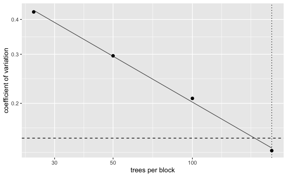
The criterion falls as a power of the block size, and the exponent is fitted rather than assumed: over four generating processes and both engines it lay between $-0.55$ and $-0.60$ with $R^2$ of at least 0.98, so it is a clean power law whose exponent is not the $-0.5$ a plain standard error would give. The answer is an ordinary integer and goes on behaving as one, so it can be handed straight back to the engine that raised the question:
required + 100L
#> [1] 300
stability() asks the same question of replicates you already hold, and
assumes nothing about where they came from.
When the matrix does not fit
Two storage forms, and they are not interchangeable.
sparsify(px, threshold = 0.05)
#> <proximity_sparse> 400 x 400
#>   engine   : randomForest
#>   trees    : 500
#>   type     : inbag
#>   threshold: 0.05
#>   stored   : 50.4% of entries
nystrom(rf, book[, predictors], landmarks = 100)
#> <proximity_nystrom> 400 x 400
#>   engine   : randomForest
#>   trees    : 500
#>   type     : inbag
#>   landmarks: 100 of 400
#>   rank     : 100
#>   stored   : 312.7 Kb against 1.2 Mb dense
sparsify() thresholds and stores the result sparsely. It saves memory
and does not survive being used: every statistic here runs on
$\sqrt{1 - P}$ or on the doubly centred matrix, and across every sample
size measured those had between 99.5 and 99.9 per cent, and exactly 100
per cent, of their entries non-zero. So the inference layer refuses a
sparse object by name rather than densifying it behind you.
nystrom() is the one that survives. It stores an $n \times r$ factor
whose cross-product is the approximation, so the $n \times n$ matrix is
never formed going in or coming out: 40 MB instead of 760 at
$n = 10{,}000$ with 500 landmarks. Its entries move much more than its
geometry does, which is the point, since the geometry is what it is for:
at $n = 400$ with 200 landmarks, 20.7 per cent relative error on the
entries and 4.9 per cent on the configuration embedding() returns.
Closing the loop with e2tree
e2tree fits a single explainable tree to the dissimilarity a forest
induces. It takes that dissimilarity as an argument, which is exactly
what this package produces, and returns a tree whose own partition comes
back as a proximity:
explanation <- e2tree::e2tree(default ~ ., data = book[, predictors],
                              D = as_dissimilarity(px), ensemble = rf)
mantel_test(px, as_proximity(explanation), n_perm = 999)$statistic
#>        r
#> 0.653591
That correlation is how much of the ensemble's geometry the single tree
reproduces, which is the question e2tree exists to answer and the one
thing it cannot ask of itself.
What the example showed
The forest arranged 400 borrowers into blocks; one of those blocks is an interaction no coefficient would have shown you. Two refits of the same forest agreed almost perfectly and a forest given two predictors instead of ten did not, so the statistic separates the cases it needs to separate. A protected attribute that the model never received still accounted for a measurable share of the arrangement. And the whole thing was checked for stability, for the number of trees it rests on, and for whether it is a kernel at all.
The theory underneath
The Gram identity. With $Z$ the stacked leaf indicator, $P = ZZ^{\top}/B$. This settles three things at once: the in-bag proximity is positive semi-definite, so $\sqrt{1-P}$ is Euclidean; the out-of-bag one is an elementwise quotient of two such products and is not; and the matrix can be computed as one sparse cross-product instead of a loop over trees. On 300 trees and 1,500 observations that is 0.16 s against 13 s.
Classical scaling and the kernel are the same computation. With
$D^2 = \mathbf{1}\mathbf{1}^{\top} - P$ and $J$ the centring operator,
$J\mathbf{1} = 0$ kills the first term and
$G = -\tfrac12 J D^2 J = \tfrac12 J P J$. So embedding() never has to
form the dissimilarity, and the same identity is what lets it read a
configuration off a Nystrom factor at $O(nr^2)$ instead of $O(n^3)$.
Permutation, not asymptotics. Every entry of a proximity matrix shares an observation with $2(n-2)$ others, so the entries are nowhere near independent and no closed-form null applies. All the tests here permute the observations, which permutes rows and columns together and preserves that dependence.
Undefined is not zero. An out-of-bag pair that was never jointly out
of bag is NA, not 0. Storing a zero would assert that the two
observations never share a leaf, when what the forest reported is that
it never had the chance to look. Every statistic is computed on the
pairs where all matrices involved are defined, and reports how many
those were.
Every exported function
as_proximity() |
the extractor, with methods for randomForest, ranger and e2tree |
as_dissimilarity(), as.dist() |
$\sqrt{1-P}$ or $1-P$ |
is_euclidean(), double_centre() |
the metric diagnostics |
make_psd() |
clip, flip or shift an indefinite proximity onto the PSD cone |
embedding() |
the classical scaling configuration, direct or from a Nystrom factor |
mantel_test(), cka(), rv_coefficient() |
compare two proximity matrices |
permanova() |
partition one across the terms of a design |
protest() |
superimpose two configurations, Procrustes |
sparsify(), nystrom() |
the two storage forms |
stability(), n_trees_required() |
how much it moves, and how many trees it takes |
autoplot() |
five methods, one per class |
loans |
the synthetic portfolio the case study runs on |
What has been measured
Four studies in inst/simulations/, seeded and re-runnable, and the
documentation quotes them rather than the other way round. Several exist
because a claim written down first turned out to be false when measured:
?sparsifysaid most pairs never share a leaf and the thresholded matrix is typically very sparse. The exact zeros are 14.3 per cent of pairs at $n = 200$ and 58.5 per cent at $n = 1600$. Replaced by the table.n_trees_required()shipped with a default ofeps = 0.01, which needs about 50,000 trees and was unreachable from any ensemble anyone would fit.- The criterion was documented as falling like $1/\sqrt{B}$. The measured exponent is $-0.56$, and the projection now fits it instead of assuming it.
- Stratified landmarks were said to help. On the whole matrix they do not at all; on the rows they were designed for they do, and only when the budget is small relative to how rare the class is.
- The seriation behind the heatmap was documented as deterministic. It is not, on a proximity: the matrix is $k/B$ and takes at most $B+1$ distinct values, so the ordering breaks the ties at random and moves with the seed.
What this does not protect you from
The proximity is a description of the model, not of the data. Everything
here is a statement about how one fitted ensemble arranges one sample; a
different forest on the same data arranges it differently, which is
precisely what stability() is for measuring rather than a caveat to be
waved away.
A Mantel correlation is not a hypothesis about the world. It tests exchangeability of the observation labels, and rejecting that null tells you the two matrices share structure, not that the structure means what you hoped.
permanova() on a proximity is a diagnostic and not a fairness
certificate. A share of variation is one number about one
representation.
And the out-of-bag proximity is not a kernel. Every method downstream
that assumes one, cka() included, refuses it rather than returning
something plausible, and make_psd() is a choice you make and not a
repair that happens to you.
Documentation
vignette("Proximum-intro"): proximity matrices as statistical objects, the in-bag and out-of-bag definitions and what separates them, the three views.vignette("comparing-forests"): the inference layer in full.vignette("large-n"): sparsification, Nystrom, stability, and how to choose.vignette("credit-scoring-case"): the three questions above, worked.
Status
Version 1.1.0, and not yet on CRAN. The roadmap is complete and the
interface is settled: extraction from randomForest, ranger and
e2tree, the transforms and the metric diagnostics, the positive
semi-definite repair, the inference layer, the scalability and stability
layers, the plots, and the streaming layer.
The stable badge is a statement about the interface rather than about
the number of users. as_proximity() was the last name to move, and it
moved so that this one would not have to; from here a breaking change
goes through a deprecation cycle. Everything 1.1.0 added is additive:
proximity_stream() is a new constructor and block_size a new
argument with a default, so nothing that ran under 1.0.0 runs
differently.
| Phase | Content | State |
|---|---|---|
| F1 | as_proximity(), the proximity object, transforms, make_psd() |
done |
| F2 | mantel_test(), cka(), rv_coefficient(), permanova(), protest() |
done |
| F3 | sparsify(), nystrom(), embedding(), stability(), n_trees_required() |
done |
| F4 | autoplot(), the vignettes, the loans data |
done |
| F5 | proximity_stream(), streamed mantel_test() and cka() |
done |
| F6 | CRAN, JSS paper | not started |
Related work
e2tree: explains a forest with a single tree built on the same similarity structure. It consumes what this package produces, andas_proximity()reads its result back.rankimp: which variables drive the representationProximumdescribes.vegan: the reference implementation of Mantel, PERMANOVA and Procrustes on ordinary dissimilarities. It cannot consume a matrix with undefined pairs, which is why this package implements them natively and usesveganonly in its tests, to check that the two agree where both apply.
References
Breiman, L. (2001). Random forests. Machine Learning, 45(1), 5-32.
Anderson, M. J. (2001). A new method for non-parametric multivariate analysis of variance. Austral Ecology, 26(1), 32-46.
McArdle, B. H. and Anderson, M. J. (2001). Fitting multivariate models to community data. Ecology, 82(1), 290-297.
Cortes, C., Mohri, M. and Rostamizadeh, A. (2012). Algorithms for learning kernels based on centered alignment. JMLR, 13, 795-828.
Williams, C. and Seeger, M. (2001). Using the Nystrom method to speed up kernel machines. NeurIPS 13.
Bar-Joseph, Z., Gifford, D. K. and Jaakkola, T. S. (2001). Fast optimal leaf ordering for hierarchical clustering. Bioinformatics, 17, S22-S29.
License
MIT, (c) Agostino Gnasso.