ConfidenceEllipse
Computation of 2D and 3D Elliptical Joint Confidence Regions
Computing elliptical joint confidence regions at a specified confidence level. It provides the flexibility to estimate either classical or robust confidence regions, which can be visualized in 2D or 3D plots. The classical approach assumes normality and uses the mean and covariance matrix to define the confidence regions. Alternatively, the robustified version employs estimators like minimum covariance determinant (MCD) and M-estimator, making them less sensitive to outliers and departures from normality. Furthermore, the functions allow users to group the dataset based on categorical variables and estimate separate confidence regions for each group. This capability is particularly useful for exploring potential differences or similarities across subgroups within a dataset. Varmuza and Filzmoser (2009, ISBN:978-1-4200-5947-2). Johnson and Wichern (2007, ISBN:0-13-187715-1). Raymaekers and Rousseeuw (2019)






The ConfidenceEllipse package computes the coordinate points of
confidence region for a given bivariate and trivariate dataset. The size
of the elliptical region is determined by the confidence level, and the
shape is determined by the covariance matrix. The confidence level is
usually chosen to be 95% or 99%, and the resulting confidence region
contains the points that are expected to lie within the multivariate
distribution.
Installation
You can install ConfidenceEllipse from CRAN using:
install.packages("ConfidenceEllipse")
Alternatively you can grab the development version from github using devtools:
install.packages("devtools")
devtools::install_github("ChristianGoueguel/ConfidenceEllipse")
Example
library(magrittr)
library(tidyselect)
library(patchwork)
library(dplyr)
library(ggplot2)
library(purrr)
library(tidyr)
library(ConfidenceEllipse)
Dataset
The dataset is comprised of 13 different measurements for 180 archaeological glass vessels from different groups (Janssen, K.H.A., De Raedt, I., Schalm, O., Veeckman, J.: Microchim. Acta 15 (suppl.) (1998) 253-267. Compositions of 15th - 17th century archaeological glass vessels excavated in Antwerp.)
data("glass", package = "ConfidenceEllipse")
glass %>% glimpse()
#> Rows: 180
#> Columns: 14
#> $ glassType <fct> 1, 1, 1, 1, 1, 1, 1, 1, 1, 1, 1, 1, 1, 1, 1, 1, 1, 1, 2, 2, …
#> $ Na2O      <dbl> 13.904, 14.194, 14.668, 14.800, 14.078, 13.600, 12.942, 15.6…
#> $ MgO       <dbl> 2.244, 2.184, 3.034, 2.455, 2.480, 1.648, 2.690, 2.028, 2.25…
#> $ Al2O3     <dbl> 1.312, 1.310, 1.362, 1.385, 1.072, 2.012, 1.420, 1.242, 1.07…
#> $ SiO2      <dbl> 67.752, 67.076, 63.254, 63.790, 68.768, 69.628, 64.012, 70.6…
#> $ P2O5      <dbl> 0.884, 0.938, 0.988, 1.200, 0.682, 0.698, 0.966, 0.210, 0.75…
#> $ SO3       <dbl> 0.052, 0.024, 0.064, 0.115, 0.070, 0.038, 0.046, 0.310, 0.03…
#> $ Cl        <dbl> 0.936, 0.966, 0.886, 0.988, 0.966, 0.908, 0.896, 0.676, 0.93…
#> $ K2O       <dbl> 3.044, 3.396, 2.828, 2.878, 2.402, 3.196, 2.526, 2.326, 2.32…
#> $ CaO       <dbl> 8.784, 8.636, 11.088, 10.833, 8.808, 6.160, 12.982, 6.324, 9…
#> $ MnO       <dbl> 0.674, 0.698, 1.240, 0.978, 0.310, 1.170, 0.874, 0.214, 0.60…
#> $ Fe2O3     <dbl> 0.364, 0.336, 0.400, 0.433, 0.242, 0.650, 0.516, 0.278, 0.25…
#> $ BaO       <dbl> 0.040, 0.040, 0.046, 0.025, 0.022, 0.156, 0.014, 0.032, 0.02…
#> $ PbO       <dbl> 0.004, 0.198, 0.134, 0.120, 0.102, 0.136, 0.120, 0.062, 0.02…
Confidence Region
Classical and robust confidence ellipses
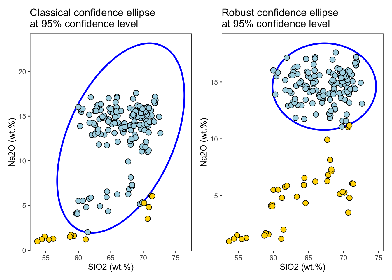
First, the confidence_ellipse function is used to compute coordinate
points of the confidence ellipse and then the ellipse is plotted on a
two-dimensional plot x and y of the data. Points that lie outside
the ellipse are considered to be outliers, while points that lie within
the ellipse are considered to be part of the underlying distribution
with the specified confidence level conf_level.
ellipse_95 <- confidence_ellipse(glass, x = SiO2, y = Na2O, conf_level = 0.95)
rob_ellipse_95 <- confidence_ellipse(glass, x = SiO2, y = Na2O, conf_level = 0.95, robust = TRUE)
ellipse_95 %>% glimpse()
#> Rows: 361
#> Columns: 2
#> $ x <dbl> 74.45896, 74.35724, 74.25314, 74.14669, 74.03792, 73.92686, 73.81356…
#> $ y <dbl> 21.99964, 22.08244, 22.16235, 22.23932, 22.31335, 22.38440, 22.45245…
cutoff <- qchisq(0.95, df = 2)
 MDsquared <- glass %>%
  select(SiO2, Na2O) %>%
  as.matrix() %>%
  mahalanobis(colMeans(.), cov(.), inverted = FALSE)
plot1 <-
  ggplot() +
  geom_path(data = ellipse_95, aes(x = x, y = y), color = "blue", linewidth = 1L) +
  geom_point(data = glass %>% mutate(md = MDsquared) %>% filter(md <= cutoff), aes(x = SiO2, y = Na2O), shape = 21L, color = "black", fill = "lightblue", size = 3L) +
  geom_point(data = glass %>% mutate(md = MDsquared) %>% filter(md > cutoff), aes(x = SiO2, y = Na2O), shape = 21L, color = "black", fill = "gold", size = 3L) +
  labs(x = "SiO2 (wt.%)", y = "Na2O (wt.%)", title = "Classical confidence ellipse\nat 95% confidence level") +
  theme_bw() +
  theme(
    panel.grid = element_blank(),
    legend.position = "none"
    )
x_mcd <- glass %>%
  select(SiO2, Na2O) %>%
  as.matrix() %>%
  robustbase::covMcd()
rob_MDsquared <- glass %>%
  select(SiO2, Na2O) %>%
  as.matrix() %>%
  mahalanobis(x_mcd$center, x_mcd$cov)
plot2 <-
  ggplot() +
  geom_path(data = rob_ellipse_95, aes(x = x, y = y), color = "blue", linewidth = 1L) +
  geom_point(data = glass %>% mutate(md = rob_MDsquared) %>% filter(md <= cutoff), aes(x = SiO2, y = Na2O), shape = 21L, color = "black", fill = "lightblue", size = 3L) +
  geom_point(data = glass %>% mutate(md = rob_MDsquared) %>% filter(md > cutoff), aes(x = SiO2, y = Na2O), shape = 21L, color = "black", fill = "gold", size = 3L) +
  labs(x = "SiO2 (wt.%)", y = "Na2O (wt.%)", title = "Robust confidence ellipse\nat 95% confidence level") +
  theme_bw() +
  theme(
    panel.grid = element_blank(),
    legend.position = "none"
    )
plot1 | plot2
Grouping
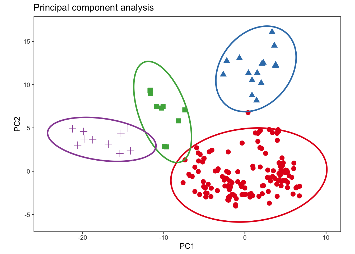
For grouping bivariate data, the .group_by argument can be used if the
data contains an unique grouping variable (.group_by = NULL by
default). When a grouping variable is provided, the function will
compute the ellipses separately for each level of the factor, allowing
you to explore potential differences or patterns within subgroups of the
data.
It’s important to note that the grouping variable should be
appropriately coded as a factor before passing it to the .group_by
argument. If the variable is currently stored as a character or numeric
type, you may need to convert it to a factor using functions like
as.factor() or forcats::as_factor().
rpca_scores <- glass %>%
  select(where(is.numeric) )%>%
  pcaPP::PCAproj(method = "qn") %>%
  pluck("scores") %>%
  as_tibble() %>%
  mutate(glassType = glass %>% pull(glassType)) %>%
  rename(PC1 = Comp.1, PC2 = Comp.2)
ellipse_pca <- rpca_scores %>% confidence_ellipse(x = PC1, y = PC2, .group_by = glassType)
ggplot() +
  geom_point(data = rpca_scores, aes(x = PC1, y = PC2, color = glassType, shape = glassType), size = 3L) +
  geom_path(data = ellipse_pca, aes(x = x, y = y, color = glassType), linewidth = 1L) +
  scale_color_brewer(palette = "Set1", direction = 1) +
  labs(x = "PC1", y = "PC2", title = "Principal component analysis") +
  theme_bw() +
  theme(
    aspect.ratio = .7,
    panel.grid = element_blank(),
    legend.position = "none"
    )
Ellipsoid
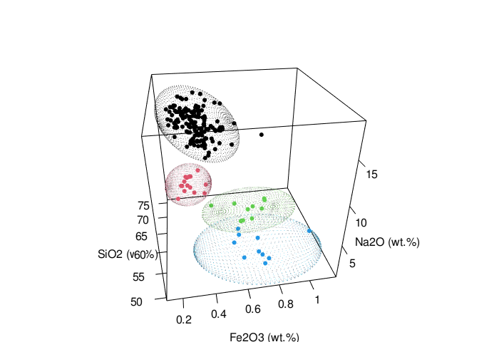
The confidence_ellipsoid function accepts an additional variable z
and computes the ellipsoid for trivariate data.
ellipsoid_grp <- glass %>% confidence_ellipsoid(SiO2, Na2O, Fe2O3, glassType)
ellipsoid_grp %>% glimpse()
#> Rows: 10,000
#> Columns: 4
#> $ x         <dbl> 67.32486, 67.32486, 67.32486, 67.32486, 67.32486, 67.32486, …
#> $ y         <dbl> 14.51964, 14.51964, 14.51964, 14.51964, 14.51964, 14.51964, …
#> $ z         <dbl> 0.5971494, 0.5971494, 0.5971494, 0.5971494, 0.5971494, 0.597…
#> $ glassType <fct> 1, 1, 1, 1, 1, 1, 1, 1, 1, 1, 1, 1, 1, 1, 1, 1, 1, 1, 1, 1, …
rgl::setupKnitr(autoprint = TRUE)
rgl::plot3d(
  x = ellipsoid_grp$x,
  y = ellipsoid_grp$y,
  z = ellipsoid_grp$z,
  xlab = "SiO2 (wt.%)",
  ylab = "Na2O (wt.%)",
  zlab = "Fe2O3 (wt.%)",
  type = "s",
  radius = 0.03,
  col = as.numeric(ellipsoid_grp$glassType)
  )
rgl::points3d(
  x = glass$SiO2,
  y = glass$Na2O,
  z = glass$Fe2O3,
  col = as.numeric(glass$glassType),
  size = 5
  )
rgl::view3d(theta = 260, phi = 30, fov = 60, zoom = .85)