Snow Profile Alignment, Aggregation, and Clustering

Snow profiles describe the vertical (1D) stratigraphy of layered snow with different layer characteristics, such as grain type, hardness, deposition date, and many more. Hence, they represent a data format similar to multivariate time series containing categorical, ordinal, and numerical data types. Use this package to align snow profiles by matching their individual layers based on Dynamic Time Warping (DTW). The aligned profiles can then be assessed with an independent, global similarity measure that is geared towards avalanche hazard assessment. Finally, through exploiting data aggregation and clustering methods, the similarity measure provides the foundation for grouping and summarizing snow profiles according to similar hazard conditions. In particular, this package allows for averaging large numbers of snow profiles with DTW Barycenter Averaging and thereby facilitates the computation of individual layer distributions and summary statistics that are relevant for avalanche forecasting purposes. For more background information refer to Herla, Horton, Mair, and Haegeli (2021) , Herla, Mair, and Haegeli (2022) , and Horton, Herla, and Haegeli (2024) .

sarp.snowprofile.alignment

The goal of sarp.snowprofile.alignment is to

align snow stratigraphy profiles by matching their individual layers based on Dynamic Time Warping (DTW)
assess the similarity of the aligned profiles with an independent similarity measure that is geared towards avalanche hazard assessment
cluster sets of snow profiles according to similar conditions based on the independent similarity measure, and
aggregate clusters of snow profiles to summarize the conditions by an average profile derived with DTW Barycenter Averaging (DBA), thereby facilitating the computation of individual layer distributions that are relevant for avalanche forecasting purposes.

Background: Snow profiles describe the vertical (1D) stratigraphy of layered snow with different layer characteristics, such as grain type, hardness, deposition/burial date, and many more. Hence, they represent a data format similar to multi-variate time series containing categorical, ordinal, and numerical data types.

Installation

You can install the CRAN release of this package with install_packages('sarp.snowprofile.alignment') or get the most recent version from our bitbucket repository with:

devtools::install_bitbucket('sfu-arp/sarp.snowprofile.alignment', ref = 'master')

Examples

Aligning pairs of snow profiles

library(sarp.snowprofile.alignment)
#> Loading required package: sarp.snowprofile

plotSPalignment(SPpairs$A_manual, SPpairs$A_modeled)

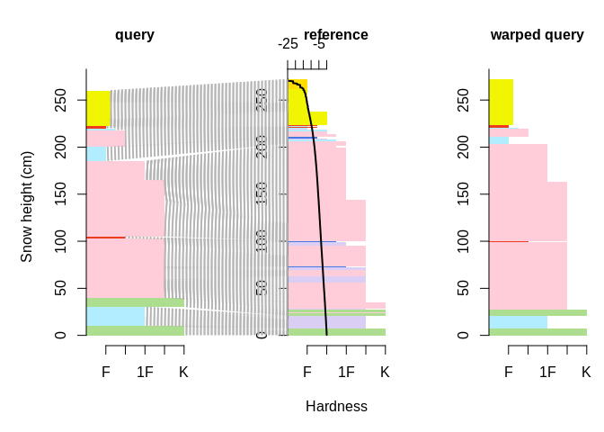
The corresponding layers between the two snow profiles query and reference have been matched, and the layer thicknesses of the query profile have been adjusted, so that the warped query is optimally aligned with the query.

Clustering snow profiles and finding a representative medoid profile

Consider a (very) short list of 5 snow profiles:

setSP <- SPgroup[c(1, 2, 5, 6, 7)]
par(mfrow = c(1, 2))
plot(setSP[[2]], main = "Profile 2")
plot(setSP, SortMethod = 'unsorted', xticklabels = "originalIndices", main = "Set of 5 profiles")

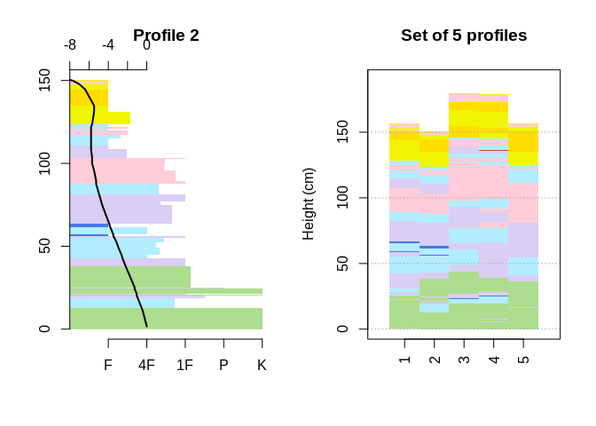
Compute the medoid snow profile that represents the group the best by aligning the profiles and assessing their similarity:

idxMedoid <- medoidSP(setSP)
paste("The most representative (medoid) profile is Profile", idxMedoid)
#> [1] "The most representative (medoid) profile is Profile 2"

The last computation told us the most representative profile from within the group is Profile 2, which we have plotted earlier.

Averaging snow profiles with DTW Barycenter Averaging

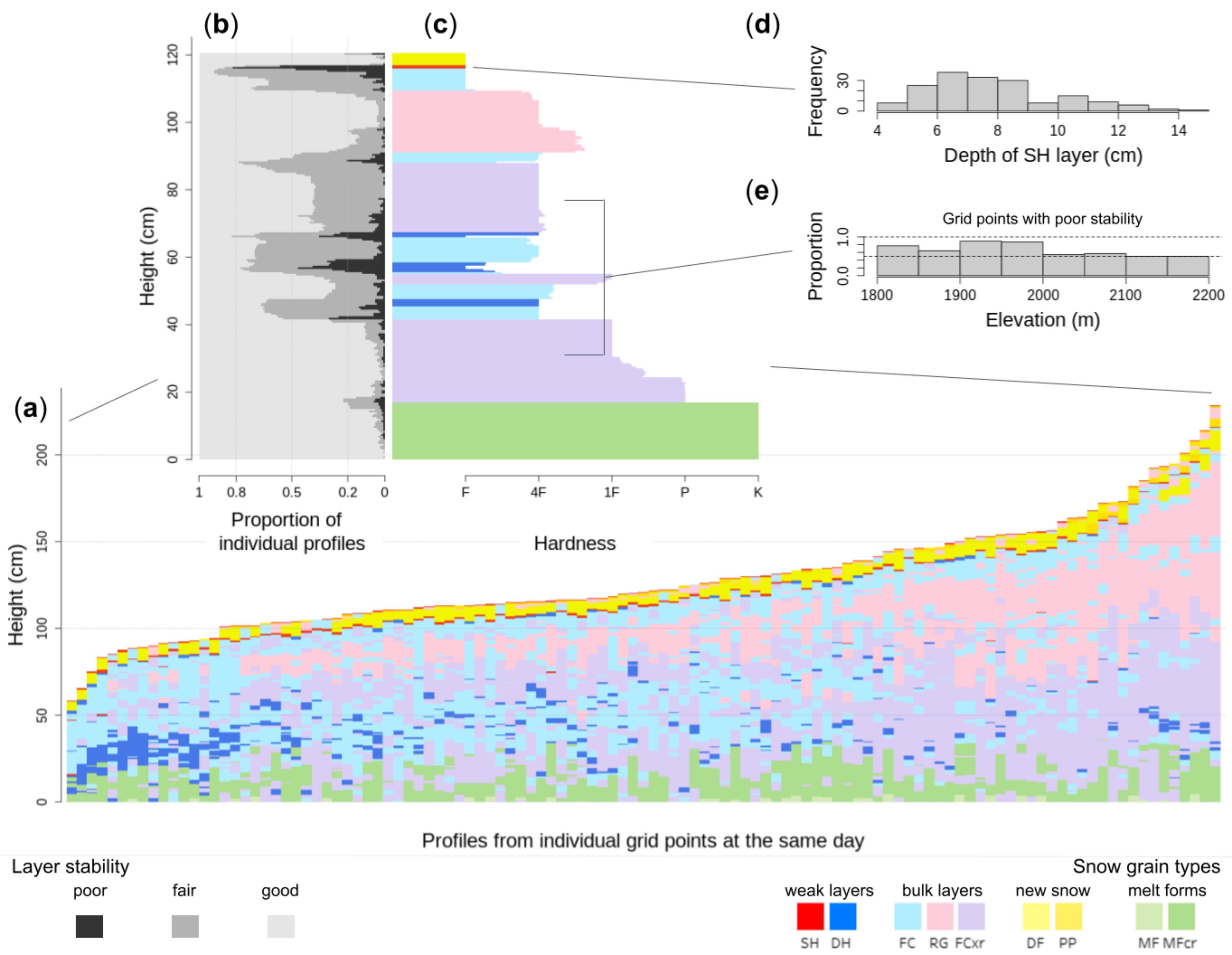
The figure shows (a) a snow profile set from an avalanche forecast region with 112 simulated profiles from the same day, (c) which is summarized by the average profile. The average profile provides access to distributions of layer and profile properties, such as e.g. (b) the distribution of layer stabilities derived from threshold sums, (d) the depth distribution of a SH layer that is starting to get buried, (e) the elevation distribution of the proportion of profiles that contain layers with poor stability in mid snowpack.

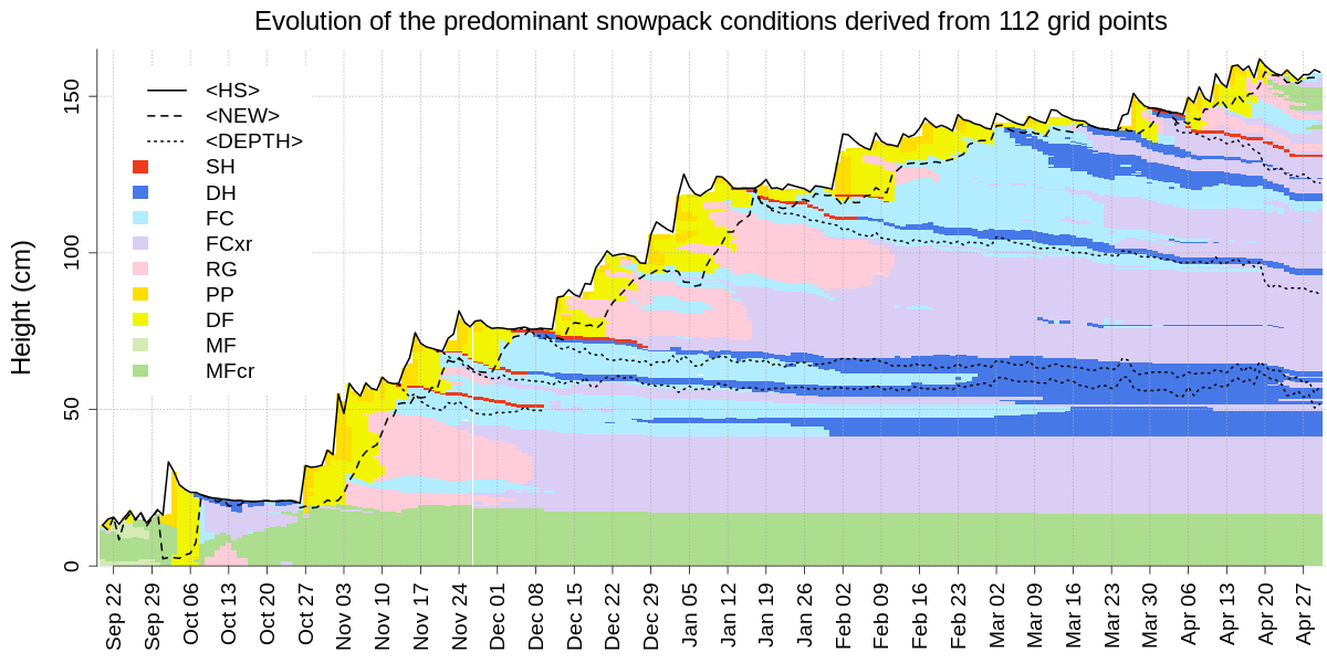
Time series of the average snow profile that illustrates the space-averaged evolution of the snow stratigraphy (visualized by snow grain types). The algorithm captures the median total snow height (solid line, ), the median amount of new snow (dashed line, ), and the median depth of several persistent weak layers (dotted lines, ).

Check out the functions averageSP, averageSPalongSeason, and backtrackLayers.

Getting started

A broader and deeper overview of the package is provided in the vignettes, cf. browseVignettes("sarp.snowprofile.alignment")). For a quick start, see ?sarp.snowprofile.alignment. This package builds on top of the general package sarp.snowprofile for data import/export and manipulation, cf. browseVignettes("sarp.snowprofile")).