netify
Tools for Network Data Workflows
Builds, validates, analyzes, and visualizes network data from
dyadic, event, matrix, 'igraph', and 'network' inputs. Supports
cross-sectional, longitudinal, bipartite, and multi-layer networks, with
conversion helpers for common modeling workflows and plotting utilities
for exploratory analysis. Network methods are described in Wasserman and
Faust (1994, ISBN:9780521387071), Cranmer et al. (2021)
netify 
Overview
netify is an R package for working with relational data. It converts edge lists, matrices, and data frames into network objects that you can analyze and visualize using a consistent set of functions.
We built netify while doing our own network research in social science. It handles common tasks like temporal network analysis, ego network extraction, and multiplex relationships without requiring multiple packages or data format conversions.
Installation
Install the package from CRAN after release:
install.packages("netify")
Install the development version from GitHub:
install.packages("devtools")
devtools::install_github("netify-dev/netify", dependencies = TRUE)
Quick Start
Transform your relational data into a network object with just one function:
library(netify)
data(icews)

# Create a network from dyadic data
icews_conflict <- netify(
  icews,
  actor1 = 'i',
  actor2 = 'j',
  time = 'year',
  symmetric = FALSE,
  weight = 'matlConf',
  nodal_vars = c('i_polity2', 'i_log_gdp', 'i_region')
)

# Print the netify object
print(icews_conflict)
✔ Network data created.
• Unipartite
• Asymmetric
• Weights from `matlConf`
• Longitudinal: 13 Periods
• # Unique Actors: 152
Network Summary Statistics (averaged across time):
          dens miss   mean recip trans
matlConf 0.113    0 12.997 0.594 0.387
• Nodal Features: i_polity2, i_log_gdp, i_region
• Dyad Features: None
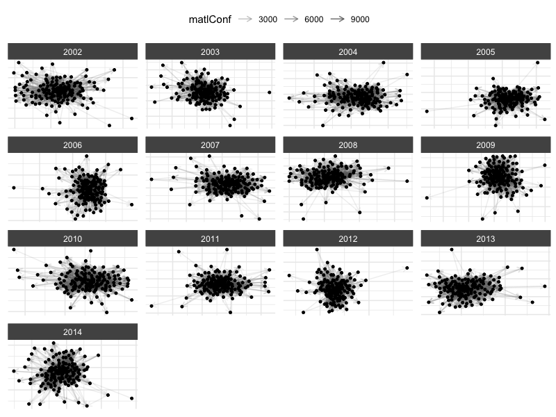
Quick visualization
# Plot the network
plot(icews_conflict)
Add node color
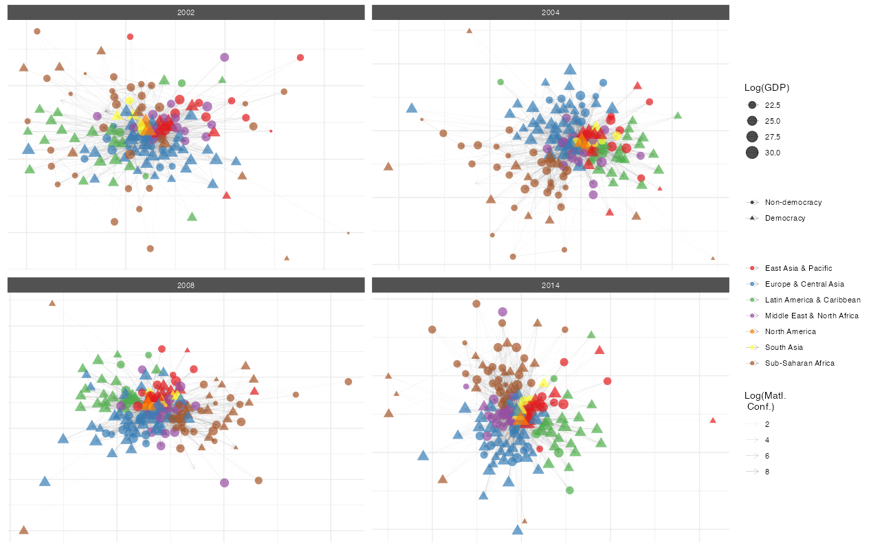
You can map node attributes to plot aesthetics:
# Create democracy indicator
icews$i_democ <- factor(
  ifelse(icews$i_polity2 >= 6, 1, 0),
  levels = c(0, 1),
  labels = c("Non-democracy", "Democracy")
)

# Add it to the network
icews_conflict <- add_node_vars(
  icews_conflict, icews,
  actor = 'i', time = 'year',
  node_vars = 'i_democ'
)

plot(
  icews_conflict,
  # Log transform weights
  mutate_weight = log1p,
  # Map node attributes to aesthetics
  node_color_by = 'i_region',
  node_size_by = 'i_log_gdp',
  node_shape_by = 'i_democ',
  # set global node alpha
  node_alpha = .7,
  # set global edge alpha
  edge_linewidth = .1,
  # Filter data
  node_filter = ~ !is.na(i_democ),
  time_filter = c('2002', '2004', '2008', '2014'),
  # clean up plot labels
  edge_alpha_label = 'Log(Matl.\n Conf.)',
  node_color_label = '',
  node_size_label = 'Log(GDP)',
  node_shape_label = ''
  ) +
  ggplot2::theme(legend.position = 'right') +
  ggplot2::scale_color_brewer(palette = 'Set1')
What can you do with a netify object?
Get network statistics
summary(icews_conflict)
This returns a data frame with network statistics for each time period:
| Year | Actors | Density | Edges | Mean Weight | Reciprocity | Transitivity |
|---|---|---|---|---|---|---|
| 2002 | 152 | 0.090 | 2069 | 1.12 | 0.200 | 0.354 |
| 2003 | 152 | 0.095 | 2193 | 1.54 | 0.294 | 0.358 |
| 2004 | 152 | 0.115 | 2666 | 1.64 | 0.647 | 0.391 |
| ... | ... | ... | ... | ... | ... | ... |
(Table shows first few rows - actual output includes all time periods)
Key functions
Building networks
netify()- Turn your data into a network objectego_netify()- Extract ego networkslayer_netify()- Stack multiple relationships into multilayer networks
Adding information
add_node_vars()- Attach attributes to actors (like GDP, democracy scores)add_dyad_vars()- Attach attributes to relationships (like trade volume, conflict events)
Wrangling networks
subset()- Pull out specific time periods or actorsmutate_weights()- Log-transform, normalize, or otherwise modify edge weights
Analysis
measurements()- Measurements of your network size and compositionsummary()- Get a quick overview of your networksummary_actor()- See how individual actors fit into the networkcompare_networks()- See how similar two networks arehomophily()- Do similar actors tend to connect?mixing_matrix()- Who connects with whom?
Visualization
plot()- Create network diagrams with sensible defaultsplot_actor_stats()- Visualize node-level statisticsplot_graph_stats()- Show how network properties change over time
Working with other packages
to_igraph()/to_network()- When you need something we don't haveto_amen()- For fitting AME or SRM modelsunnetify()- Get back to a regular data frame
Quick Reference
Essential Functions
| Task | Function | Example |
|---|---|---|
| Create network | netify() |
netify(data, actor1="from", actor2="to") |
| Extract ego network | ego_netify() |
ego_netify(net, ego="USA") |
| Create multilayer | layer_netify() |
layer_netify(list(net1, net2)) |
| Add node data | add_node_vars() |
add_node_vars(net, node_df, actor="id") |
| Add dyad data | add_dyad_vars() |
add_dyad_vars(net, dyad_df, actor1="from", actor2="to") |
| Subset network | subset() |
subset(net, time="2020") |
| Get graph level summary statistics | summary() |
summary(net) |
| Get actor level summary statistics | summary_actor() |
summary_actor(net) |
| Test homophily | homophily() |
homophily(net, attribute="democracy", method="correlation") |
| Create mixing matrix | mixing_matrix() |
mixing_matrix(net, attribute="regime_type", normalized=TRUE) |
| Test dyadic correlations | dyad_correlation() |
dyad_correlation(net, dyad_vars="geographic_distance") |
| Attribute report | attribute_report() |
attribute_report(net, node_vars=c("region", "democracy"), dyad_vars="distance") |
| Compare networks | compare_networks() |
compare_networks(list(net1, net2), method="all") |
| Plot network | plot() |
plot(net) |
| Convert to igraph | to_igraph() |
g <- to_igraph(net) |
| Convert to statnet/network | to_statnet() |
g <- to_statnet(net) |
| Convert to amen | to_amen() |
amen_data <- to_amen(net) |
| Back to data frame | unnetify() |
df <- unnetify(net) |
Scaling to large networks
netify stores adjacencies as dense matrices/arrays, which keeps the API uniform but makes memory the binding constraint at large N (a single dense N x N slice costs 8 * N^2 bytes; e.g. ~7.6 MB at N=1K, ~191 MB at N=5K, and ~1.7 GB at N=15K). A few knobs and benchmarks to keep in mind:
- Sparse matrix guard. Passing a
Matrix::sparseMatrix(e.g.dgCMatrix) tonetify()densifies internally. WhenN > 5000and density is under 1%,netify()aborts with a guidance message rather than silently allocating gigabytes. Override withforce_dense = TRUEif you really want the dense object, or build from an edgelistdata.frameto skip the matrix intermediate entirely. - Fast actor stats.
summary_actor()defaults tostats = "all"(degree + closeness + betweenness + eigenvector + HITS). The closeness/betweenness paths dominate wall-clock at large N, so atN >= getOption("netify.fast_threshold", 1500L)netify auto-promotes the default call tostats = "fast", which returns only the degree- and strength-style columns. Passstats = "all"explicitly to force centralities, or raise the threshold viaoptions(netify.fast_threshold = ...). - Indicative timings (single laptop core, directed weighted toy nets):
| N | edges | netify() |
summary() |
summary_actor(fast) |
to_igraph() |
|---|---|---|---|---|---|
| 1000 | ~10K | 0.08 s | 0.6 s | 0.6 s | 0.1 s |
| 5000 | ~50K | 0.8 s | 4.8 s | 4.5 s | 0.6 s |
For 10K+ actor / weekly-slice workflows, prefer edgelist inputs, set stats = "fast" explicitly, and consider to_igraph() for any heavy centrality work.
When you might need something else
netify covers common network data workflows and provides converters for specialized packages when you need methods outside its scope:
- Statistical models: Use
to_amen()for latent factor models orto_statnet()for ERGMs - Graph algorithms: Convert with
to_igraph()to use igraph methods - Custom analysis: Use
unnetify()to return to a data frame
These converters let you move between netify and other network-analysis tools without rebuilding the data by hand.
Getting help
- Browse installed vignettes with
browseVignettes("netify"); additional workflow articles are on the package website. - Check function documentation:
?netify,?plot.netify, etc. - Report bugs: GitHub Issues
Citation
If you use netify in your research, please cite:
citation("netify")
Contributors
netify is developed by:
- Cassy Dorff (Vanderbilt University)
- Shahryar Minhas (Michigan State University)
With contributions from:
- Ha Eun Choi (Michigan State University)
- Colin Henry (Vanderbilt University)
- Tosin Salau (Michigan State University)
This work is supported by National Science Foundation Awards #2017162 and #2017180.
License
GPL-3
Made for the network analysis community