Tidy, 'ggplot2'-Native Visualization for Genomic Variants

A simple, opinionated toolkit for visualizing genomic variant data using a 'ggplot2'-native grammar. Accepts VCF files or plain data frames and produces lollipop plots, consequence summaries, mutational spectrum charts, and cohort-level comparisons as standard 'ggplot2' objects. Designed for both wet-lab biologists and experienced bioinformaticians.

ggvariant

ggvariant reads variant data from a VCF file or a plain data frame and produces ggplot2 plots for common tasks in variant review: lollipop plots of variant position along a gene, consequence summaries by sample or gene, mutational spectrum charts, and cohort-level comparisons such as oncoprints and per-sample mutation burden. Every function accepts either input format and returns a standard ggplot object, so the result composes with any ggplot2 layer, scale, or theme you already use. Designed for both wet-lab biologists and experienced bioinformaticians.

Installation

Install the released version from CRAN:

install.packages("ggvariant")

Install the development version from GitHub:

# install.packages("remotes")
remotes::install_github("josh45-source/ggvariant")

Example

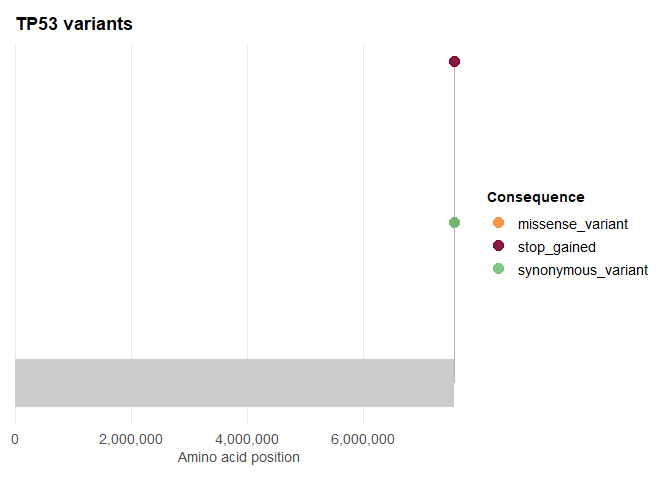
Read a VCF file and plot variant positions along a gene:

library(ggvariant)

vcf_file <- system.file("extdata", "example.vcf", package = "ggvariant")
variants <- read_vcf(vcf_file)

plot_lollipop(variants, gene = "TP53")

If your data is already in a data frame — a spreadsheet export, say, rather than a VCF file — coerce_variants() maps your column names onto the same tidy format instead.

Overview

• Reading and coercing variants — read_vcf() parses VCF v4.x files, including gzipped and multi-sample files, and extracts SnpEff (ANN) or VEP (CSQ) annotations automatically. coerce_variants() remaps an existing data frame’s columns onto the same format.
• Plots — plot_lollipop(), plot_consequence_summary(), plot_variant_spectrum(), plot_oncoprint() (also plot_waterfall(), an alias for the same function), and plot_tmb().
• Palettes and themes — gv_palette() and theme_ggvariant() expose the built-in colours and plot theme for reuse in plots you build yourself.

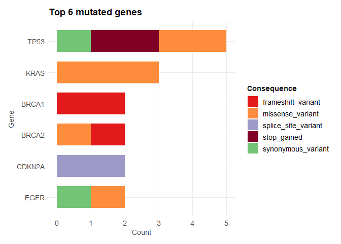
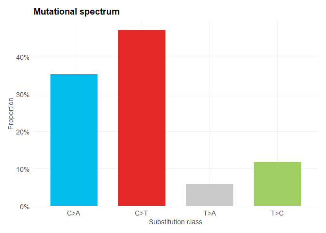
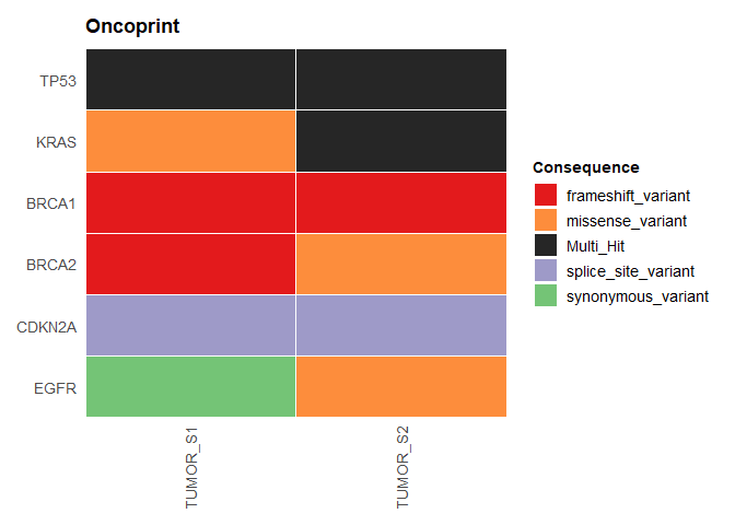
A few of the other plot types, on the same example data:

plot_consequence_summary(variants, group_by = "gene", top_n = 6)

plot_variant_spectrum(variants)

plot_oncoprint(variants, top_n = 6)

See vignette("ggvariant") for a full walkthrough — domain annotations, colouring by sample, proportional and faceted views, interactive plotly output — or the function reference for argument details.

Customisation

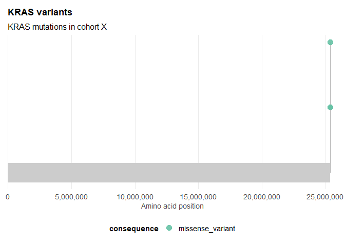
Every function returns a standard ggplot object, so any ggplot2 layer, scale, or theme composes onto it directly:

library(ggplot2)

plot_lollipop(variants, gene = "KRAS") +
  scale_colour_brewer(palette = "Set2") +
  theme(legend.position = "bottom") +
  labs(subtitle = "KRAS mutations in cohort X")

Package structure

ggvariant/
├── R/
│   ├── ggvariant-package.R       # Package documentation
│   ├── read_vcf.R                # read_vcf() and coerce_variants()
│   ├── plot_lollipop.R           # plot_lollipop()
│   ├── plot_functions.R          # plot_consequence_summary(), plot_variant_spectrum()
│   └── utils.R                   # Theme, palettes, shared helpers
├── tests/
│   └── testthat/
│       └── test-core.R           # Unit tests
├── inst/
│   └── extdata/
│       └── example.vcf           # Bundled example VCF
├── DESCRIPTION
└── NAMESPACE

Roadmap

• [ ] plot_oncoprint() — sample × gene mutation matrix
• [ ] plot_copy_number() — CNV segment visualisation
• [ ] plot_rainfall() — kataegis / mutation density along genome
• [ ] plot_tmb() — tumour mutation burden comparison across cohorts
• [ ] BSgenome integration for automatic trinucleotide context extraction
• [ ] Shiny module for non-coding users

Contributing

Pull requests are welcome. Please open an issue first to discuss proposed changes. All contributions should include tests.

Acknowledgements

The waterfall/oncoprint visualisation in v0.2.0 was suggested by Dr Nour-al-dain Marzouka.

License

MIT

Citation

If you use ggvariant in your research, please cite:

Ayo, J. J. (2026). ggvariant: Tidy, ggplot2-native visualization for genomic variants (R package version 0.1.0). CRAN. https://doi.org/10.32614/CRAN.package.ggvariant