Geographic Networks

Provides classes and methods for handling networks or graphs whose nodes are geographical (i.e. locations in the globe). The functionality includes the creation of objects of class geonetwork as a graph with node coordinates, the computation of network measures, the support of spatial operations (projection to different Coordinate Reference Systems, handling of bounding boxes, etc.) and the plotting of the geonetwork object combined with supplementary cartography for spatial representation.

geonetwork

Classes and methods for handling networks or graphs whose nodes are geographical (i.e. locations in the globe). Create, transform, plot.

Installation

You can install the released version of geonetwork from CRAN with:

install.packages("geonetwork")

Alternatively, install the latest development version with:

install.packages("geonetwork", repos = 'https://cirad-astre.r-universe.dev')

Example

Creation

A geonetwork is an object of class igraph whose nodes have geospatial attributes (i.e. coordinates and CRS).

Consider the distances (in km) between 21 cities in Europe from the datasets package. A simple way of constructing a geonetwork is by combining a data.frame of nodes with one of edges:

## Use OpenStreetMap's Nominatim service through the package {tmaptools}
## to retrieve coordinates of the cities.
## Restrict search to Europe (to prevent homonym cities to show up)
cities <- tmaptools::geocode_OSM(
  paste(
    labels(datasets::eurodist),
    "viewbox=-31.64063%2C60.93043%2C93.16406%2C31.65338",
    sep = "&"
  )
)
cities$city <- labels(datasets::eurodist)

distances <- 
  expand.grid(
    origin = labels(datasets::eurodist),
    destin = labels(datasets::eurodist),
    stringsAsFactors = FALSE,
    KEEP.OUT.ATTRS = FALSE
  )
distances <- 
  cbind(
    distances[distances$destin < distances$origin,],
    distance = as.numeric(datasets::eurodist)
  )

str(cities)
#> 'data.frame':    21 obs. of  8 variables:
#>  $ query  : chr  "Athens&viewbox=-31.64063%2C60.93043%2C93.16406%2C31.65338" "Barcelona&viewbox=-31.64063%2C60.93043%2C93.16406%2C31.65338" "Brussels&viewbox=-31.64063%2C60.93043%2C93.16406%2C31.65338" "Calais&viewbox=-31.64063%2C60.93043%2C93.16406%2C31.65338" ...
#>  $ lat    : num  38 41.4 50.8 51 49.5 ...
#>  $ lon    : num  23.73 2.18 4.35 1.85 -1.58 ...
#>  $ lat_min: num  37.8 41.3 50.8 50.9 49.3 ...
#>  $ lat_max: num  38.1 41.5 50.9 51 49.7 ...
#>  $ lon_min: num  23.57 2.05 4.31 1.81 -1.96 ...
#>  $ lon_max: num  23.89 2.23 4.44 1.93 -1.14 ...
#>  $ city   : chr  "Athens" "Barcelona" "Brussels" "Calais" ...
str(distances)
#> 'data.frame':    210 obs. of  3 variables:
#>  $ origin  : chr  "Barcelona" "Brussels" "Calais" "Cherbourg" ...
#>  $ destin  : chr  "Athens" "Athens" "Athens" "Athens" ...
#>  $ distance: num  3313 2963 3175 3339 2762 ...

eurodist <- geonetwork(
  distances,
  nodes = cities[, c("city", "lon", "lat")], 
  directed = FALSE
)

Several assumptions were made here unless otherwise specified:

• The first column in cities was matched with the first two columns in distances.

• The second and third columns in cities were assumed to be longitude and latitude in decimal degrees in a WGS84 CRS.

• The remaining column in distances was treated as an edge weight.

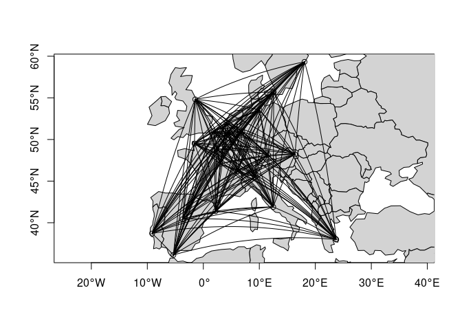
Now we can readily plot the network, optionally with some additional geographical layer for context:

## Base system
plot(eurodist, axes = TRUE, type = "n")
plot(sf::st_geometry(spData::world), col = "lightgray", add = TRUE)
plot(eurodist, axes = TRUE, add = TRUE)