Shed Light on Black Box Machine Learning Models

Shed light on black box machine learning models by the help of model performance, variable importance, global surrogate models, ICE profiles, partial dependence (Friedman J. H. (2001) ), accumulated local effects (Apley D. W. (2016) ), further effects plots, interaction strength, and variable contribution breakdown (Gosiewska and Biecek (2019) ). All tools are implemented to work with case weights and allow for stratified analysis. Furthermore, multiple flashlights can be combined and analyzed together.

{flashlight}

Overview

The goal of this package is shed light on black box machine learning models.

The main props of {flashlight}:

1. It is simple, yet flexible.
2. It offers model agnostic tools like model performance, variable importance, global surrogate models, ICE profiles, partial dependence, ALE, and further effects plots, scatter plots, interaction strength, and variable contribution breakdown/SHAP for single observations.
3. It allows to assess multiple models side-by-side.
4. It supports "group by" operations.
5. It works with case weights.

Currently, models with numeric or binary response are supported.

Installation

# From CRAN
install.packages("flashlight")

# Development version
devtools::install_github("mayer79/flashlight")

Usage

Let's start with an iris example. For simplicity, we do not split the data into training and testing/validation sets.

library(ggplot2)
library(MetricsWeighted)
library(flashlight)

fit_lm <- lm(Sepal.Length ~ ., data = iris)

# Make explainer object
fl_lm <- flashlight(
  model = fit_lm, 
  data = iris, 
  y = "Sepal.Length", 
  label = "lm",               
  metrics = list(RMSE = rmse, `R-squared` = r_squared)
)

Performance

fl_lm |> 
  light_performance() |> 
  plot(fill = "darkred") +
  labs(x = NULL, title = "Performance on training data")

fl_lm |> 
  light_performance(by = "Species") |> 
  plot(fill = "darkred") +
  ggtitle("Performance split by Species")

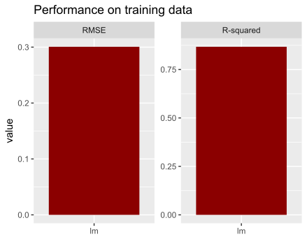
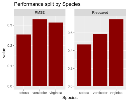
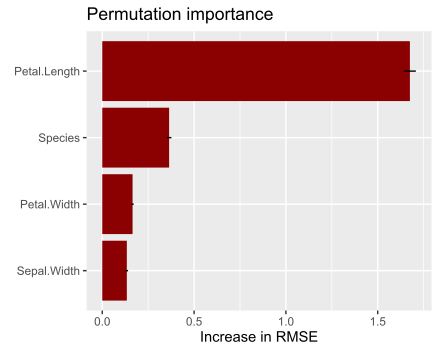
Permutation importance regarding first metric

Error bars represent standard errors, i.e., the uncertainty of the estimated importance.

fl_lm |>
  light_importance(m_repetitions = 4) |> 
  plot(fill = "darkred") +
  labs(title = "Permutation importance", y = "Increase in RMSE")

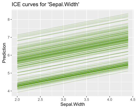
ICE curves for Petal.Width

fl_lm |> 
  light_ice("Sepal.Width", n_max = 200) |> 
  plot(alpha = 0.3, color = "chartreuse4") +
  labs(title = "ICE curves for 'Sepal.Width'", y = "Prediction")

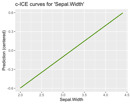
fl_lm |> 
  light_ice("Sepal.Width", n_max = 200, center = "middle") |> 
  plot(alpha = 0.3, color = "chartreuse4") +
  labs(title = "c-ICE curves for 'Sepal.Width'", y = "Prediction (centered)")

PDPs

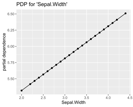
fl_lm |> 
  light_profile("Sepal.Width", n_bins = 40) |> 
  plot() +
  ggtitle("PDP for 'Sepal.Width'")

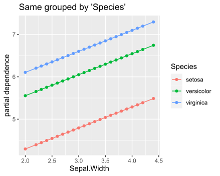
fl_lm |> 
  light_profile("Sepal.Width", n_bins = 40, by = "Species") |> 
  plot() +
  ggtitle("Same grouped by 'Species'")

2D PDP

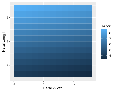
fl_lm |> 
  light_profile2d(c("Petal.Width", "Petal.Length")) |> 
  plot()

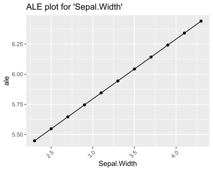
ALE

fl_lm |> 
  light_profile("Sepal.Width", type = "ale") |> 
  plot() +
  ggtitle("ALE plot for 'Sepal.Width'")

Different profile plots in one

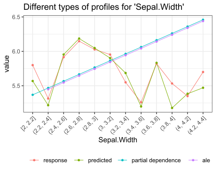
fl_lm |> 
  light_effects("Sepal.Width") |> 
  plot(use = "all") +
  ggtitle("Different types of profiles for 'Sepal.Width'")

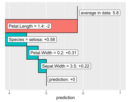
Variable contribution breakdown for single observation

fl_lm |> 
  light_breakdown(new_obs = iris[1, ]) |> 
  plot()

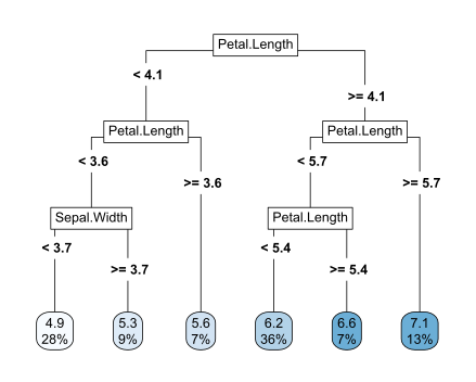
Global surrogate tree

fl_lm |> 
  light_global_surrogate() |> 
  plot()

Multiple models

Multiple flashlights can be combined to a multiflashlight.

library(rpart)

fit_tree <- rpart(
  Sepal.Length ~ ., 
  data = iris, 
  control = list(cp = 0, xval = 0, maxdepth = 5)
)

# Make explainer object
fl_tree <- flashlight(
  model = fit_tree, 
  data = iris, 
  y = "Sepal.Length", 
  label = "tree",               
  metrics = list(RMSE = rmse, `R-squared` = r_squared)
)

# Combine with other explainer
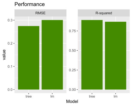
fls <- multiflashlight(list(fl_tree, fl_lm))

fls |> 
  light_performance() |> 
  plot(fill = "chartreuse4") +
  labs(x = "Model", title = "Performance")

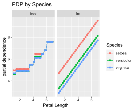
fls |> 
  light_profile("Petal.Length", n_bins = 40, by = "Species") |> 
  plot() +
  ggtitle("PDP by Species")

More

Check out the vignette for more information and important references.