Calculating Optimum Sampling Effort in Community Ecology

A system for calculating the optimal sampling effort, based on the ideas of "Ecological cost-benefit optimization" as developed by A. Underwood (1997, ISBN 0 521 55696 1). Data is obtained from simulated ecological communities with prep_data() which formats and arranges the initial data, and then the optimization follows the following procedure of four functions: (1) prep_data() takes the original dataset and creates simulated sets that can be used as a basis for estimating statistical power and type II error. (2) sim_beta() is used to estimate the statistical power for the different sampling efforts specified by the user. (3) sim_cbo() calculates then the optimal sampling effort, based on the statistical power and the sampling costs. Additionally, (4) scompvar() calculates the variation components necessary for (5) Underwood_cbo() to calculate the optimal combination of number of sites and samples depending on either an economic budget or on a desired statistical accuracy. Lastly, (6) plot_power() helps the user visualize the results of sim_beta().

ecocbo

Calculating Optimum Sampling Effort in Community Ecology

ecocbo is an R package that helps scientists calculate the optimum sampling effort for community ecology projects. The package is based on the principles developed in the SSP package, which simulates ecological communities by extracting and using parameters that control the simulation. The simulated communities are then compared with PERMANOVA to estimate their components of variation and consequently the optimal sampling effort.

ecocbo is a valuable tool for scientists who need to design efficient sampling plans. The package can help scientists to save time and money by ensuring that they collect the minimum amount of data necessary to achieve their research goals.

Installation

You can easily obtain ‘ecocbo’ from CRAN:

install.packages("ecocbo")

Alternatively, you can install the development version of ecocbo from GitHub:

install.packages("devtools")
devtools::install_github("arturoSP/ecocbo")

Example

This is a basic example which shows you how to use the different functions in the package:

Prepare the data

# Load data and pre-process it.
data(epiDat)

simResults <- prep_data(data = epiDat, 
                        type = "counts", Sest.method = "average",
                        cases = 5, N = 100, M = 10,
                        n = 5, m = 5, k = 30,
                        transformation = "none", method = "bray",
                        dummy = FALSE, useParallel = FALSE,
                        model = "single.factor")

Calculate components of variation.

compVar <- scompvar(data = simResults)
compVar
#>     Source Est.var.comp
#> 1 Residual     0.331926

Calculate statistical power

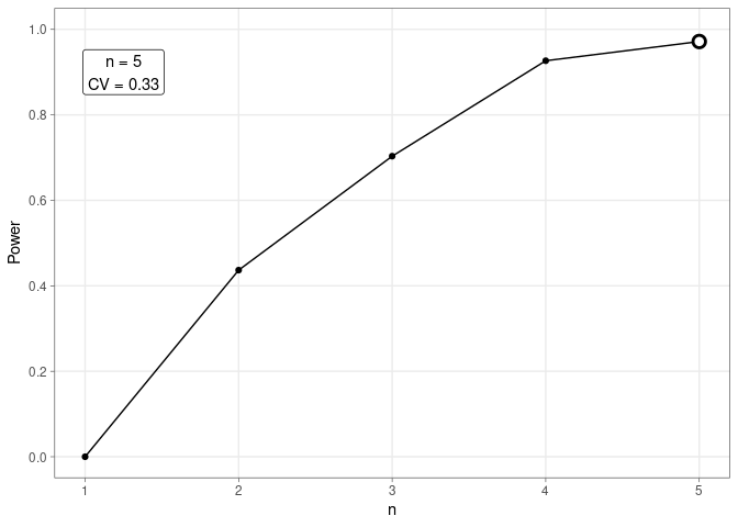
betaResult <- sim_beta(simResults, alpha = 0.05)
betaResult
#> Power at different sampling efforts (n):
#>       Power
#> n = 2  0.44
#> n = 3  0.70
#> n = 4  0.93
#> n = 5  0.97

Determine optimal sampling effort

The sampling effort can be evaluated depending on an economic budget (ct) or desired precision level (multSE), depending on the proposed parameter, the function will calculate optimal values for number of treatments (bOpt) and replicates (nOpt).

cboCost <- sim_cbo(betaResult, cn = 75)
cboCost
#> Sampling designs that meet the required power:
#>  n     Power Cost Suggested
#>  2 0.4366667  150          
#>  3 0.7033333  225          
#>  4 0.9266667  300          
#>  5 0.9716194  375       ***
#> 
#> The listed cost is per treatment.

Additionally…

Plot the power progression as sampling increases.

# This plot will look different in every simulation
plot_power(data = betaResult, n = NULL, method = "power")

R packages required for running ecocbo

• Required: SSP, ggplot2, ggpubr, sampling, stats, rlang, foreach, parallel, doParallel, doSNOW, vegan, plotly

• Suggested: knitr, rmarkdown, testthat

Participating institutions