Functions for Tidy Analysis and Generation of Random Data

To make it easy to generate random numbers based upon the underlying stats distribution functions. All data is returned in a tidy and structured format making working with the data simple and straight forward. Given that the data is returned in a tidy 'tibble' it lends itself to working with the rest of the 'tidyverse'.

TidyDensity

The goal of {TidyDensity} is to make working with random numbers from different distributions easy. All tidy_ distribution functions provide the following components:

• [r_]
• [d_]
• [q_]
• [p_]

Installation

You can install the released version of {TidyDensity} from CRAN with:

install.packages("TidyDensity")

And the development version from GitHub with:

# install.packages("devtools")
devtools::install_github("spsanderson/TidyDensity")

Example

This is a basic example which shows you how to solve a common problem:

library(TidyDensity)
library(dplyr)
library(ggplot2)

tidy_normal()
#> # A tibble: 50 × 7
#>    sim_number     x       y    dx       dy      p       q
#>    <fct>      <int>   <dbl> <dbl>    <dbl>  <dbl>   <dbl>
#>  1 1              1 -1.87   -3.51 0.000235 0.0307 -1.87  
#>  2 1              2 -0.839  -3.37 0.000617 0.201  -0.839 
#>  3 1              3  0.580  -3.22 0.00147  0.719   0.580 
#>  4 1              4 -0.0620 -3.07 0.00322  0.475  -0.0620
#>  5 1              5  0.360  -2.92 0.00644  0.641   0.360 
#>  6 1              6 -0.165  -2.78 0.0118   0.434  -0.165 
#>  7 1              7 -1.65   -2.63 0.0201   0.0494 -1.65  
#>  8 1              8 -0.277  -2.48 0.0315   0.391  -0.277 
#>  9 1              9  1.77   -2.34 0.0461   0.961   1.77  
#> 10 1             10  0.604  -2.19 0.0628   0.727   0.604 
#> # ℹ 40 more rows

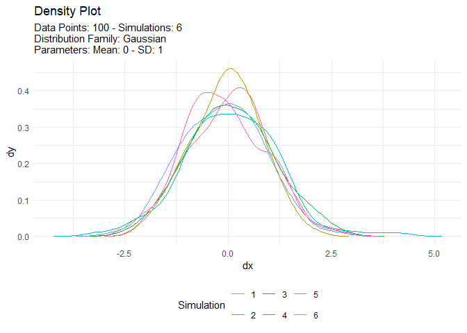
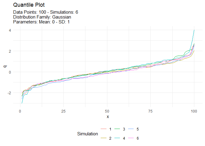
An example plot of the tidy_normal data.

tn <- tidy_normal(.n = 100, .num_sims = 6)

tidy_autoplot(tn, .plot_type = "density")

tidy_autoplot(tn, .plot_type = "quantile")

tidy_autoplot(tn, .plot_type = "probability")

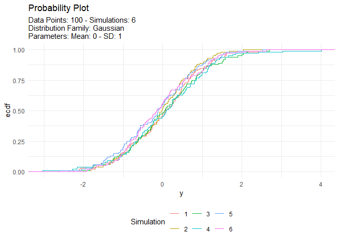
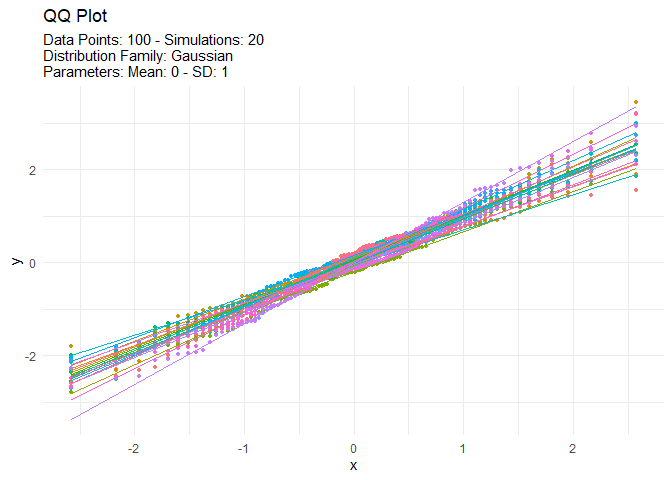
tidy_autoplot(tn, .plot_type = "qq")

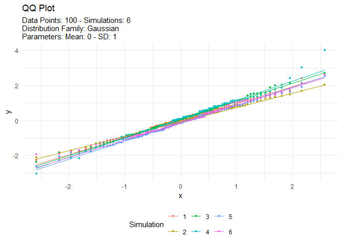
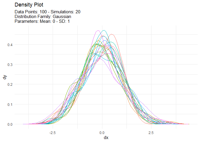
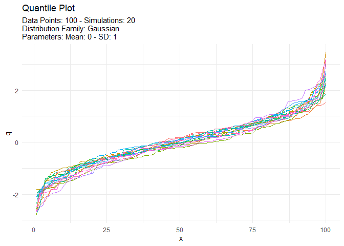
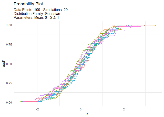
We can also take a look at the plots when the number of simulations is greater than nine. This will automatically turn off the legend as it will become too noisy.

tn <- tidy_normal(.n = 100, .num_sims = 20)

tidy_autoplot(tn, .plot_type = "density")

tidy_autoplot(tn, .plot_type = "quantile")

tidy_autoplot(tn, .plot_type = "probability")

tidy_autoplot(tn, .plot_type = "qq")