RCDT
Fast 2D Constrained Delaunay Triangulation
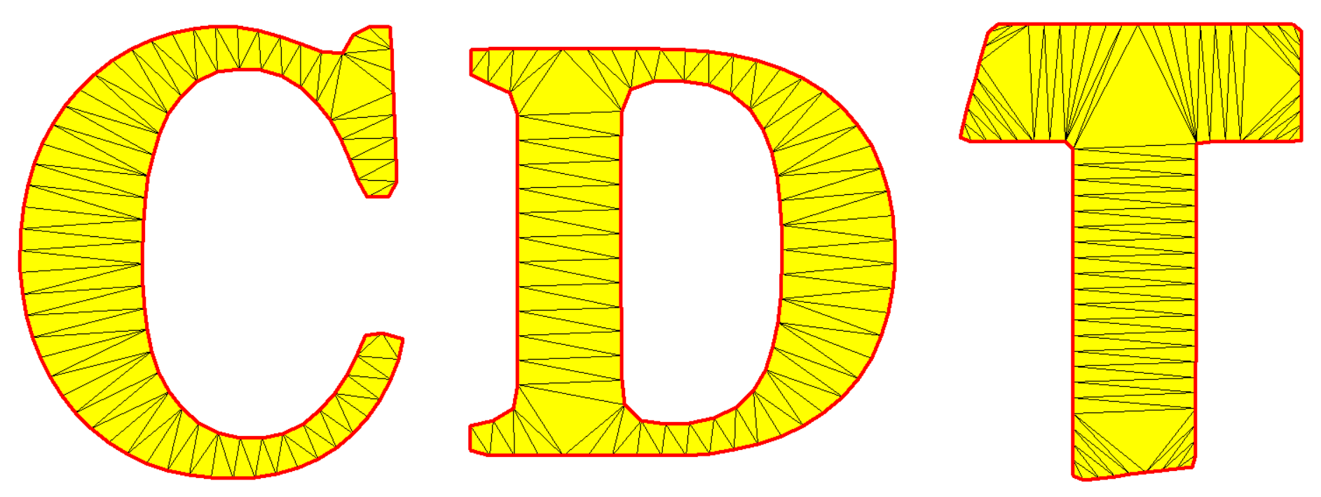
Performs 2D Delaunay triangulation, constrained or unconstrained, with the help of the C++ library 'CDT'. A function to plot the triangulation is provided. The constrained Delaunay triangulation has applications in geographic information systems.
The ‘RCDT’ package - constrained 2D Delaunay triangulation

The pentagram
# vertices
R <- sqrt((5-sqrt(5))/10)     # outer circumradius
r <- sqrt((25-11*sqrt(5))/10) # circumradius of the inner pentagon
X <- R * vapply(0L:4L, function(i) cos(pi/180 * (90+72*i)), numeric(1L))
Y <- R * vapply(0L:4L, function(i) sin(pi/180 * (90+72*i)), numeric(1L))
x <- r * vapply(0L:4L, function(i) cos(pi/180 * (126+72*i)), numeric(1L))
y <- r * vapply(0L:4L, function(i) sin(pi/180 * (126+72*i)), numeric(1L))
vertices <- rbind(
  c(X[1L], Y[1L]),
  c(x[1L], y[1L]),
  c(X[2L], Y[2L]),
  c(x[2L], y[2L]),
  c(X[3L], Y[3L]),
  c(x[3L], y[3L]),
  c(X[4L], Y[4L]),
  c(x[4L], y[4L]),
  c(X[5L], Y[5L]),
  c(x[5L], y[5L])
)
# edge indices (pairs)
edges <- cbind(1L:10L, c(2L:10L, 1L))
# constrained Delaunay triangulation
library(RCDT)
del <- delaunay(vertices, edges)
# plot
opar <- par(mar = c(0, 0, 0, 0))
plotDelaunay(
  del, type = "n", asp = 1, fillcolor = "distinct", lwd_borders = 3,
  xlab = NA, ylab = NA, axes = FALSE
)
par(opar)
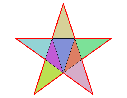
# area
delaunayArea(del)
## [1] 0.3102707
sqrt(650 - 290*sqrt(5)) / 4 # exact value
## [1] 0.3102707
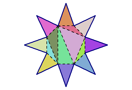
An eight-pointed star
I found its vertices with the Julia library Luxor.
vertices <- rbind(
  c(2.121320343559643, 2.1213203435596424),
  c(0.5740251485476348, 1.38581929876693),
  c(0.0, 3.0),
  c(-0.5740251485476346, 1.38581929876693),
  c(-2.1213203435596424, 2.121320343559643),
  c(-1.38581929876693, 0.5740251485476349),
  c(-3.0, 0.0),
  c(-1.3858192987669302, -0.5740251485476345),
  c(-2.121320343559643, -2.1213203435596424),
  c(-0.5740251485476355, -1.3858192987669298),
  c(0.0, -3.0),
  c(0.574025148547635, -1.38581929876693),
  c(2.121320343559642, -2.121320343559643),
  c(1.3858192987669298, -0.5740251485476355),
  c(3.0, 0.0),
  c(1.38581929876693, 0.5740251485476349)
)
# edge indices
edges <- cbind(1L:16L, c(2L:16L, 1L))
library(RCDT)
del <- delaunay(vertices, edges)
opar <- par(mar = c(0, 0, 0, 0))
plotDelaunay(
  del, type = "n", asp = 1, fillcolor = "distinct",
  col_borders = "navy", lty_edges = 2, lwd_borders = 3, lwd_edges = 2,
  xlab = NA, ylab = NA, axes = FALSE
)
par(opar)
Triangulation of a polygon with a hole
n <- 100L # outer number of sides
angles1 <- seq(0, 2*pi, length.out = n + 1L)[-1L]
outer_points <- cbind(cos(angles1), sin(angles1))
m <- 10L  # inner number of sides
angles2 <- seq(0, 2*pi, length.out = m + 1L)[-1L]
inner_points <- 0.5 * cbind(cos(angles2), sin(angles2))
points <- rbind(outer_points, inner_points)
# constraint edges
indices <- 1L:n
edges_outer <- cbind(
  indices, c(indices[-1L], indices[1L])
)
indices <- n + 1L:m
edges_inner <- cbind(
  indices, c(indices[-1L], indices[1L])
)
edges <- rbind(edges_outer, edges_inner)
# constrained Delaunay triangulation
del <- delaunay(points, edges)
# plot
opar <- par(mar = c(0, 0, 0, 0))
plotDelaunay(
  del, type = "n", asp = 1, lwd_borders = 3, col_borders = "black",
  fillcolor = "random", col_edges = "yellow",
  axes = FALSE, xlab = NA, ylab = NA
)
par(opar)
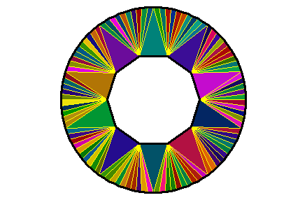
One can also enter a vector of colors in the fillcolor argument.
First, see the number of triangles:
del[["mesh"]]
##  mesh3d object with 110 vertices, 110 triangles.
There are 110 triangles. Let’s make a cyclic vector of 110 colors:
colors <- viridisLite::viridis(55)
colors <- c(colors, rev(colors))
And let’s plot now:
opar <- par(mar = c(0, 0, 0, 0))
plotDelaunay(
  del, type = "n", asp = 1, lwd_borders = 3, col_borders = "black",
  fillcolor = colors, col_edges = "black", lwd_edges = 1.5,
  axes = FALSE, xlab = NA, ylab = NA
)
par(opar)
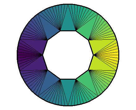
The colors are assigned to the triangles in the order they are given, but only after the triangles have been circularly ordered.
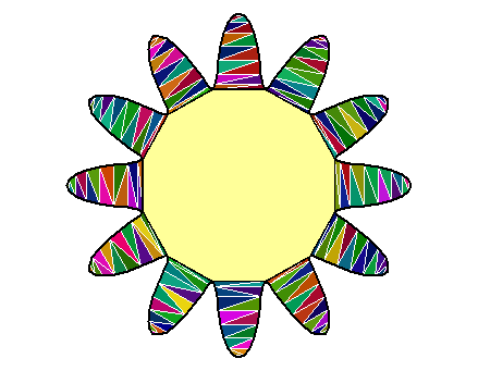
A funny curve
I found this curve here.
t_ <- seq(-pi, pi, length.out = 193L)[-1L]
r_ <- 0.1 + 5*sqrt(cos(6*t_)^2 + 0.7^2)
xy <- cbind(r_*cos(t_), r_*sin(t_))
edges1 <- cbind(1L:192L, c(2L:192L, 1L))
inner <- which(r_ == min(r_))
edges2 <- cbind(inner, c(tail(inner, -1L), inner[1L]))
del <- delaunay(xy, edges = rbind(edges1, edges2))
opar <- par(mar = c(0, 0, 0, 0))
plotDelaunay(
  del, type = "n", col_borders = "black", lwd_borders = 2,
  fillcolor = "random", col_edges = "white",
  axes = FALSE, xlab = NA, ylab = NA, asp = 1
)
polygon(xy[inner, ], col = "#ffff99")
par(opar)
License
The ‘RCDT’ package as a whole is distributed under GPL-3 (GNU GENERAL PUBLIC LICENSE version 3).
It uses the C++ library CDT which is permissively licensed under MPL-2.0. A copy of the ‘CDT’ license is provided in the file LICENSE.note, and the source code of this library can be found in the src folder.