JMH
Joint Model of Heterogeneous Repeated Measures and Survival Data
Maximum likelihood estimation for the semi-parametric joint modeling of competing risks and longitudinal data in the presence of heterogeneous within-subject variability, proposed by Li and colleagues (2023)
JMH

The JMH package jointly models both mean trajectory and within-subject
variability of the longitudinal biomarker together with the (competing
risks) survival outcome.
Installation
You can install the development version of JMH from GitHub with:
# install.packages("devtools")
devtools::install_github("shanpengli/JMH")
Declaration
This is the final release of the JMH package. Active development has
been moved to the FastJM package, which provides improved
functionality and ongoing support. Users are strongly encouraged to
transition to FastJM.
Example
The JMH package comes with several simulated datasets. To fit a joint
model, we use JMMLSM function.
library(JMH)
data(ydata)
data(cdata)
## fit a joint model
fit <- JMMLSM(cdata = cdata, ydata = ydata,
              long.formula = Y ~ Z1 + Z2 + Z3 + time,
              surv.formula = Surv(survtime, cmprsk) ~ var1 + var2 + var3,
              variance.formula = ~ Z1 + Z2 + Z3 + time,
              quadpoint = 6, random = ~ 1|ID, print.para = FALSE)
fit
#>
#> Call:
#>  JMMLSM(cdata = cdata, ydata = ydata, long.formula = Y ~ Z1 + Z2 + Z3 + time, surv.formula = Surv(survtime, cmprsk) ~ var1 + var2 + var3, variance.formula = ~Z1 + Z2 + Z3 + time, random = ~1 | ID, quadpoint = 6, print.para = FALSE)
#>
#> Data Summary:
#> Number of observations: 1353
#> Number of groups: 200
#>
#> Proportion of competing risks:
#> Risk 1 : 45.5 %
#> Risk 2 : 32.5 %
#>
#> Numerical intergration:
#> Method:  adaptive Guass-Hermite quadrature
#> Number of quadrature points:  6
#>
#> Model Type: joint modeling of longitudinal continuous and competing risks data with the presence of intra-individual variability
#>
#> Model summary:
#> Longitudinal process: Mixed effects location scale model
#> Event process: cause-specific Cox proportional hazard model with non-parametric baseline hazard
#>
#> Loglikelihood:  -3621.603
#>
#> Fixed effects in mean of longitudinal submodel:  Y ~ Z1 + Z2 + Z3 + time
#>
#>             Estimate      SE   Z value  p-val
#> (Intercept)  4.85342 0.12451  38.97918 0.0000
#> Z1           1.55235 0.16535   9.38841 0.0000
#> Z2           1.93774 0.14598  13.27409 0.0000
#> Z3           1.09289 0.05321  20.53796 0.0000
#> time         4.01129 0.02978 134.71376 0.0000
#>
#> Fixed effects in variance of longitudinal submodel:  log(sigma^2) ~ Z1 + Z2 + Z3 + time
#>
#>             Estimate      SE  Z value  p-val
#> (Intercept)  0.50745 0.12838  3.95260 0.0001
#> Z1           0.50509 0.16005  3.15590 0.0016
#> Z2          -0.42508 0.13781 -3.08463 0.0020
#> Z3           0.14405 0.04494  3.20563 0.0013
#> time         0.09050 0.02422  3.73720 0.0002
#>
#> Survival sub-model fixed effects:  Surv(survtime, cmprsk) ~ var1 + var2 + var3
#>
#>        Estimate      SE Z value  p-val
#> var1_1  1.09710 0.32647 3.36051 0.0008
#> var2_1  0.19237 0.26154 0.73553 0.4620
#> var3_1  0.49611 0.08908 5.56951 0.0000
#>
#> var1_2 -0.88311 0.33702 -2.62037 0.0088
#> var2_2  0.80905 0.30127  2.68549 0.0072
#> var3_2  0.20871 0.09312  2.24143 0.0250
#>
#> Association parameters:
#>                   Estimate      SE  Z value  p-val
#> (Intercept)_1      0.97480 0.62808  1.55202 0.1207
#> (Intercept)_2     -0.18580 0.47949 -0.38750 0.6984
#> var_(Intercept)_1  0.50030 0.58190  0.85977 0.3899
#> var_(Intercept)_2 -0.84481 0.52520 -1.60857 0.1077
#>
#>
#> Random effects:
#>   Formula: ~1 | ID
#>                             Estimate      SE Z value  p-val
#> (Intercept)                  0.49542 0.11339 4.36913 0.0000
#> var_(Intercept)              0.45581 0.11129 4.09578 0.0000
#> (Intercept):var_(Intercept)  0.26738 0.07854 3.40429 0.0007
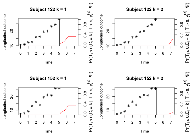
The JMH package can make dynamic prediction given the longitudinal
history information. Below is a toy example for competing risks data.
Conditional cumulative incidence probabilities for each failure will be
presented.
cnewdata <- cdata[cdata$ID %in% c(122, 152), ]
ynewdata <- ydata[ydata$ID %in% c(122, 152), ]
survfit <- survfitJMMLSM(fit, seed = 100, ynewdata = ynewdata, cnewdata = cnewdata,
                         u = seq(5.2, 7.2, by = 0.5), Last.time = "survtime",
                         obs.time = "time", method = "GH")
survfit
#>
#> Prediction of Conditional Probabilities of Event
#> based on the  adaptive  Guass-Hermite quadrature rule with 6 quadrature points
#> $`122`
#>      times       CIF1      CIF2
#> 1 5.069089 0.00000000 0.0000000
#> 2 5.200000 0.05596021 0.0000000
#> 3 5.700000 0.14584944 0.0000000
#> 4 6.200000 0.33882152 0.0000000
#> 5 6.700000 0.33882152 0.0000000
#> 6 7.200000 0.33882152 0.2171424
#>
#> $`152`
#>      times      CIF1       CIF2
#> 1 5.133665 0.0000000 0.00000000
#> 2 5.200000 0.0517717 0.00000000
#> 3 5.700000 0.1357406 0.00000000
#> 4 6.200000 0.3195265 0.00000000
#> 5 6.700000 0.3195265 0.00000000
#> 6 7.200000 0.3195265 0.06007945
oldpar <- par(mfrow = c(2, 2), mar = c(5, 4, 4, 4))
plot(survfit, include.y = TRUE)
par(oldpar)
If we assess the prediction accuracy of the fitted joint model using
Brier score as a calibration measure, we may run PEJMMLSM to calculate
the Brier score.
PE <- PEJMMLSM(fit, seed = 100, landmark.time = 3, horizon.time = c(4:6),
               obs.time = "time", method = "GH",
               n.cv = 3)
#> The 1 th validation is done!
#> The 2 th validation is done!
#> The 3 th validation is done!
summary(PE, error = "Brier")
#>
#> Expected Brier Score at the landmark time of 3
#> based on 3 fold cross validation
#>   Horizon Time Brier Score 1 Brier Score 2
#> 1            4    0.06369906    0.06194668
#> 2            5    0.10838731    0.11052099
#> 3            6    0.20187572    0.11613515
An alternative tool is to run MAEQJMMLSM to calculate the prediction
error by comparing the predicted and empirical risks stratified on
different risk groups based on quantile of the predicted risks.
## evaluate prediction accuracy of fitted joint model using cross-validated mean absolute prediction error
MAEQ <- MAEQJMMLSM(fit, seed = 100, landmark.time = 3,
                   horizon.time = c(4:6),
                   obs.time = "time", method = "GH", n.cv = 3)
#> The 1 th validation is done!
#> The 2 th validation is done!
#> The 3 th validation is done!
summary(MAEQ)
#>
#> Sum of absolute error across quintiles of predicted risk scores at the landmark time of 3
#> based on 3 fold cross validation
#>   Horizon Time  CIF1  CIF2
#> 1            4 0.386 0.262
#> 2            5 0.476 0.346
#> 3            6 0.456 0.430
Using area under the ROC curve (AUC)/concordance index (C-index) as a
discrimination measure, we may run AUCJMMLSM to calculate the
AUC/C-index score.
AUC <- AUCJMMLSM(fit, seed = 100, landmark.time = 3, horizon.time = c(4:6),
               obs.time = "time", method = "GH", metric = "AUC",
               n.cv = 3)
#> The 1 th validation is done!
#> The 2 th validation is done!
#> The 3 th validation is done!
summary(AUC)
#>
#> Expected AUC at the landmark time of 3
#> based on 3 fold cross validation
#>   Horizon Time      AUC1      AUC2
#> 1            4 0.5502137 0.6839226
#> 2            5 0.6182312 0.6523506
#> 3            6 0.6103724 0.7065657

Cindex <- AUCJMMLSM(fit, seed = 100, landmark.time = 3, horizon.time = c(4:6),
               obs.time = "time", method = "GH", metric = "Cindex",
               n.cv = 3)
#> The 1 th validation is done!
#> The 2 th validation is done!
#> The 3 th validation is done!
summary(Cindex)
#>
#> Expected Cindex at the landmark time of 3
#> based on 3 fold cross validation
#>   Horizon Time   Cindex1   Cindex2
#> 1            4 0.6154102 0.6509733
#> 2            5 0.6132650 0.6463436
#> 3            6 0.6125965 0.6463436