Modern Graphs for Design of Experiments with 'ggplot2'

Generate commonly used plots in the field of design of experiments using 'ggplot2'. 'ggDoE' currently supports the following plots: alias matrix, box cox transformation, boxplots, lambda plot, regression diagnostic plots, half normal plots, main and interaction effect plots for factorial designs, contour plots for response surface methodology, Pareto plot, and two dimensional projections of a latin hypercube design.

ggDoE

Installation

You can install:

• the latest release from CRAN with

install.packages('ggDoE')

• the development version from GitHub with

if (!require("pak")) install.packages("pak")
pak::pak("toledo60/ggDoE")

Overview

With ggDoE you’ll be able to generate common plots used in Design of Experiments with ggplot2.

library(ggDoE)

The following plots are currently available:

1. Alias Matrix
2. Box-Cox Transformation
3. Lambda Plot
4. Boxplots
5. Regression Diagnostic Plots
6. Half-Normal Plot
7. Interaction Effects Plot for a Factorial Design
8. Main Effects Plot for a Factorial Design
9. Contour Plots for Response Surface Methodology
10. Pareto Plot
11. Two Dimensional Projections of a Latin Hypercube Design

The following datasets/designs are included in ggDoE as tibbles:

• adapted_epitaxial: Adapted epitaxial layer experiment obtain from the book
  “Experiments: Planning, Analysis, and Optimization, 2nd Edition”

• original_epitaxial: Original epitaxial layer experiment obtain from the book
  “Experiments: Planning, Analysis, and Optimization, 2nd Edition”

• pulp_experiment: Reflectance Data, Pulp Experiment obtain from the book
  “Experiments: Planning, Analysis, and Optimization, 2nd Edition”

• girder_experiment: Girder experiment obtain from the book
  “Experiments: Planning, Analysis, and Optimization, 2nd Edition”

• aliased_design: D-efficient minimal aliasing design obtained from the article
  “Efficient Designs With Minimal Aliasing by Bradley Jones and Christopher J. Nachtsheim”

Citation

If you want to cite this package in a scientific journal or in any other context, run the following code in your R console

citation('ggDoE')

Warning in citation("ggDoE"): could not determine year for 'ggDoE' from package
DESCRIPTION file

To cite package 'ggDoE' in publications use:

  Toledo Luna J (????). _ggDoE: Modern Graphs for Design of Experiments
  with 'ggplot2'_. R package version 0.8, <https://ggdoe.netlify.app>.

A BibTeX entry for LaTeX users is

  @Manual{,
    title = {ggDoE: Modern Graphs for Design of Experiments with 'ggplot2'},
    author = {Jose {Toledo Luna}},
    note = {R package version 0.8},
    url = {https://ggdoe.netlify.app},
  }

Contributing to the package

I welcome feedback, suggestions, issues, and contributions! Check out the CONTRIBUTING file for more details.

Examples of Plots

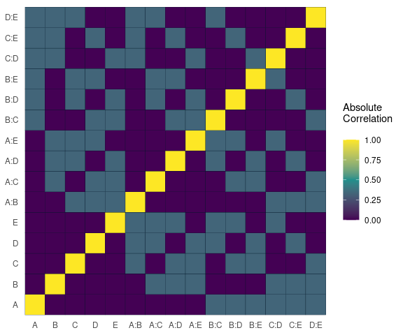
Alias Matrix

Correlation matrix plot to visualize the Alias matrix

alias_matrix(design=aliased_design)

Box-Cox Transformation

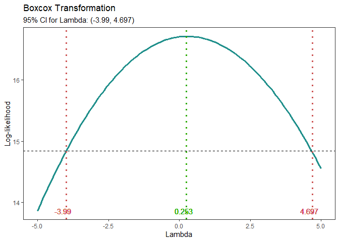
model <- lm(s2 ~ (A+B+C+D),data = adapted_epitaxial)
boxcox_transform(model,lambda = seq(-5,5,0.2))

Lambda Plot

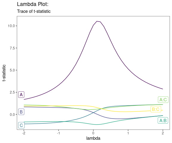
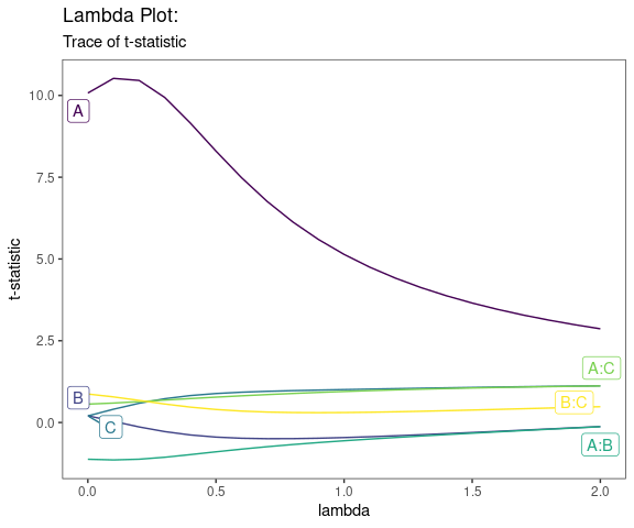
Obtain the trace plot of the t-statistics after applying Boxcox transformation across a specified sequence of lambda values

model <-  lm(s2 ~ (A+B+C)^2,data=original_epitaxial)
lambda_plot(model)

lambda_plot(model, lambda = seq(0,2,by=0.1))

Boxplots

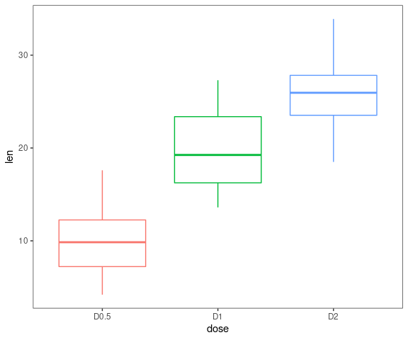
data <- ToothGrowth
data$dose <- factor(data$dose,levels = c(0.5, 1, 2),
                    labels = c("D0.5", "D1", "D2"))

gg_boxplots(data,y = 'len',x = 'dose')

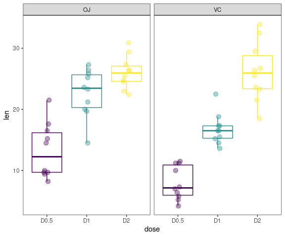
gg_boxplots(data,y = 'len',x = 'dose',
            group_var = 'supp',
            color_palette = 'viridis',
            jitter_points = TRUE)

Regression Diagnostic Plots

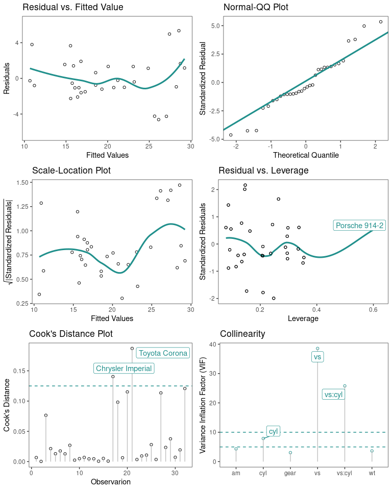
1. Residual vs. Fitted Values
2. Normal-QQ plot
3. Scale-Location plot
4. Residual vs. Leverage
5. Cook’s Distance
6. Collinearity

The default plots are 1-4

model <- lm(mpg ~ wt + am + gear + vs * cyl, data = mtcars)
gg_lm(model,which_plots=1:6)

Half-Normal Plot

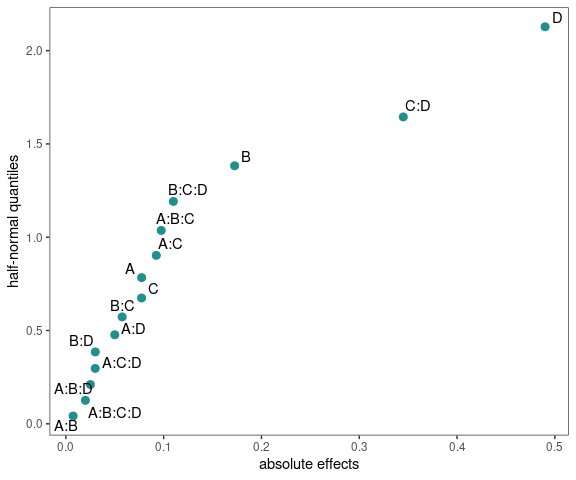
model <- lm(ybar ~ (A+B+C+D)^4,data=adapted_epitaxial)
half_normal(model)

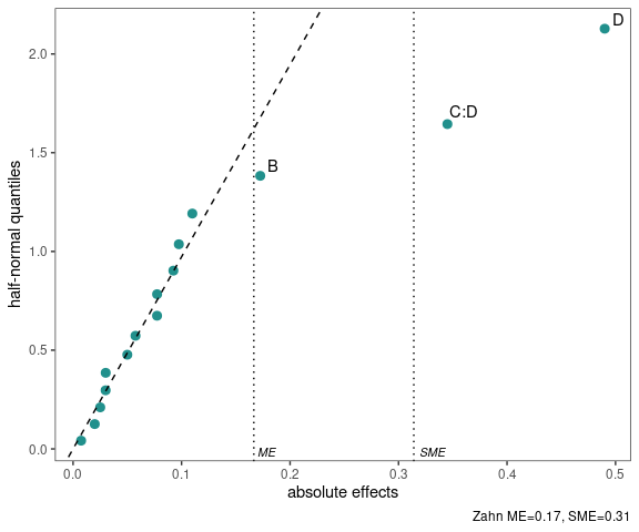
half_normal(model,method='Zahn',alpha=0.1,
            ref_line=TRUE,label_active=TRUE,
            margin_errors=TRUE)

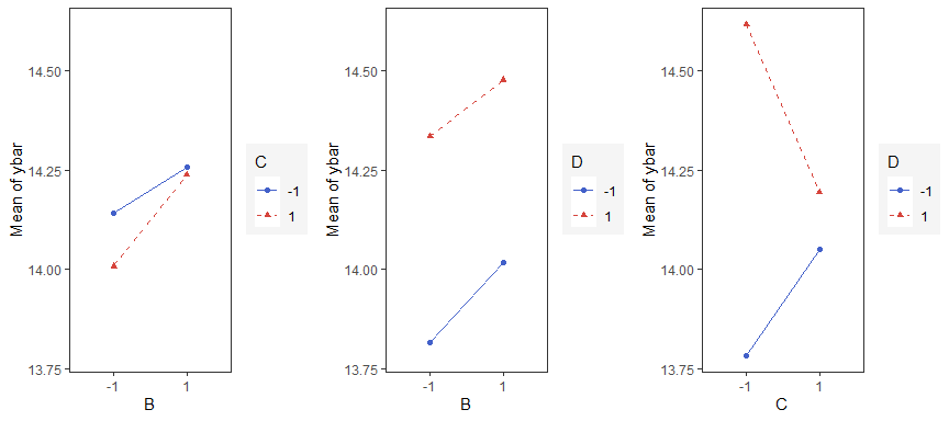
Interaction Effects Plot

Interaction effects plot between two factors in a factorial design

interaction_effects(adapted_epitaxial,response = 'ybar',
                    exclude_vars = c('s2','lns2'))

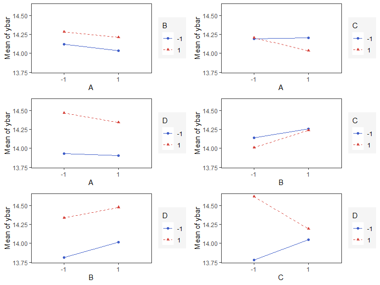
interaction_effects(adapted_epitaxial,response = 'ybar',
                    exclude_vars = c('A','s2','lns2'),
                    n_columns=3)

Main Effects Plots

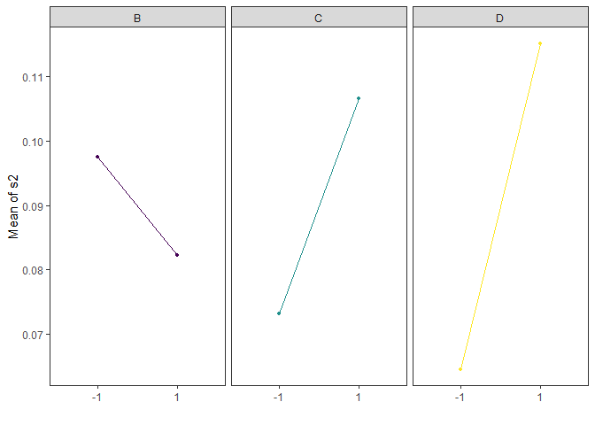
Main effect plots for each factor in a factorial design

main_effects(original_epitaxial,
             response='s2',
             exclude_vars = c('A','ybar','lns2'),
             color_palette = 'viridis',
             n_columns=3)

Contour Plots

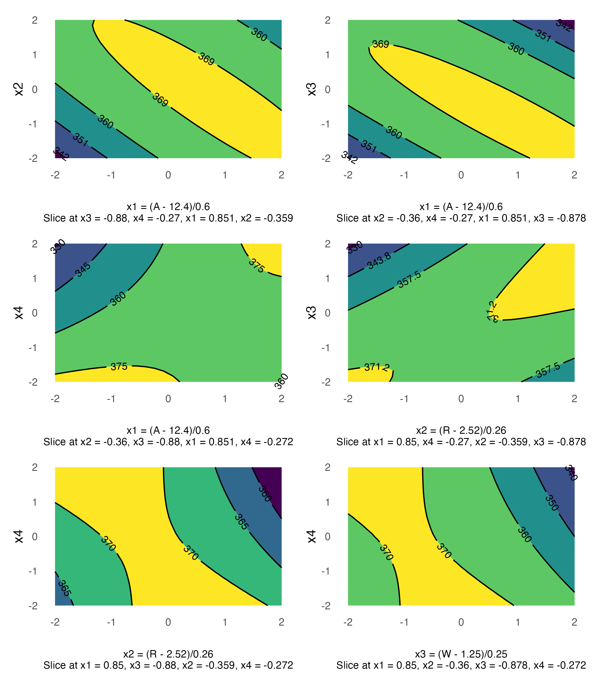
contour plot(s) that display the fitted surface for an rsm object involving two or more numerical predictors

heli.rsm <- rsm::rsm(ave ~ SO(x1, x2, x3, x4), 
                     data = rsm::heli)

gg_rsm(heli.rsm,formula = ~x1+x2+x3+x4,
       at = rsm::xs(heli.rsm))

Pareto Plot

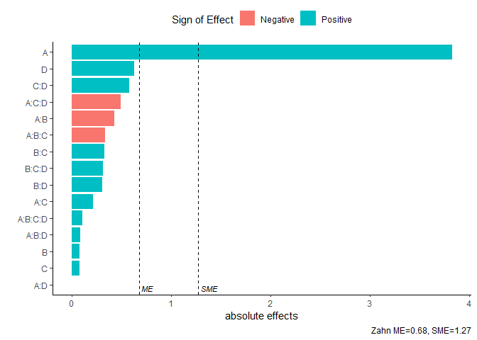
Pareto plot of effects with cutoff values for the margin of error (ME) and simultaneous margin of error (SME)

model <- lm(lns2 ~ (A+B+C+D)^4,data=original_epitaxial)
pareto_plot(model)

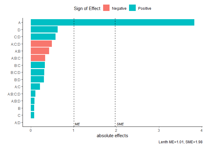
pareto_plot(model,method='Zahn',alpha=0.1)

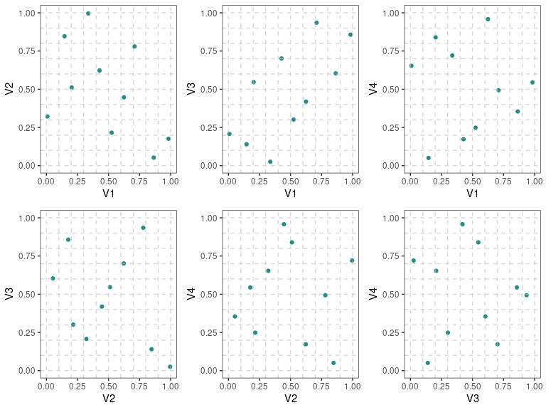
Two Dimensional Projections

This function will output all two dimensional projections from a Latin hypercube design

set.seed(10)
X <- lhs::randomLHS(n=10, k=4)
pair_plots(X,n_columns=3,grid = TRUE)