Two-Stage Difference-in-Differences Following Gardner (2021)

Estimates Two-way Fixed Effects difference-in-differences/event-study models using the approach proposed by Gardner (2021) . To avoid the problems caused by OLS estimation of the Two-way Fixed Effects model, this function first estimates the fixed effects and covariates using untreated observations and then in a second stage, estimates the treatment effects.

did2s

The goal of did2s is to estimate TWFE models without running into the problem of staggered treatment adoption.

For common issues, see this issue: https://github.com/kylebutts/did2s/issues/12

Installation

You can install did2s from CRAN with:

install.packages("did2s")

To install the development version, run the following:

devtools::install_github("kylebutts/did2s")

Two-stage Difference-in-differences (Gardner 2021)

For details on the methodology, view this vignette

To view the documentation, type ?did2s into the console.

The main function is did2s which estimates the two-stage did procedure. This function requires the following options:

• yname: the outcome variable
• first_stage: formula for first stage, can include fixed effects and covariates, but do not include treatment variable(s)!
• second_stage: This should be the treatment variable or in the case of event studies, treatment variables.
• treatment: This has to be the 0/1 treatment variable that marks when treatment turns on for a unit. If you suspect anticipation, see note above for accounting for this.
• cluster_var: Which variables to cluster on

Optional options:

• weights: Optional variable to run a weighted first- and second-stage regressions
• bootstrap: Should standard errors be bootstrapped instead? Default is False.
• n_bootstraps: How many clustered bootstraps to perform for standard errors. Default is 250.

did2s returns a list with two objects:

1. fixest estimate for the second stage with corrected standard errors.

TWFE vs. Two-Stage DID Example

I will load example data from the package and plot the average outcome among the groups.

# Automatically loads fixest
library(did2s)
#> Loading required package: fixest
#> did2s (v1.1.0). For more information on the methodology, visit <https://www.kylebutts.github.io/did2s>
#> 
#> To cite did2s in publications use:
#> 
#>   Butts & Gardner, "The R Journal: did2s: Two-Stage
#>   Difference-in-Differences", The R Journal, 2022
#> 
#> A BibTeX entry for LaTeX users is
#> 
#>   @Manual{,
#>     title = {did2s: Two-Stage Difference-in-Differences Following Gardner (2021)},
#>     author = {Kyle Butts and John Gardner},
#>     year = {2021},
#>     url = {https://journal.r-project.org/articles/RJ-2022-048/},
#>   }

# Load Data from R package
data("df_het", package = "did2s")
df_het = as.data.frame(df_het)

Here is a plot of the average outcome variable for each of the groups:

# Mean for treatment group-year
agg <- aggregate(df_het$dep_var, by = list(g = df_het$g, year = df_het$year), FUN = mean)

agg$g <- as.character(agg$g)
agg$g <- ifelse(agg$g == "0", "Never Treated", agg$g)

never <- agg[agg$g == "Never Treated", ]
g1 <- agg[agg$g == "2000", ]
g2 <- agg[agg$g == "2010", ]


plot(0, 0,
  xlim = c(1990, 2020), ylim = c(3.5, 7.2), type = "n",
  main = "Data-generating Process", ylab = "Outcome", xlab = "Year"
)
abline(v = c(1999.5, 2009.5), lty = 2)
lines(never$year, never$x, col = "#8e549f", type = "b", pch = 15)
lines(g1$year, g1$x, col = "#497eb3", type = "b", pch = 17)
lines(g2$year, g2$x, col = "#d2382c", type = "b", pch = 16)
legend(
  x = 1990, y = 7.1, col = c("#8e549f", "#497eb3", "#d2382c"),
  pch = c(15, 17, 16),
  legend = c("Never Treated", "2000", "2010")
)

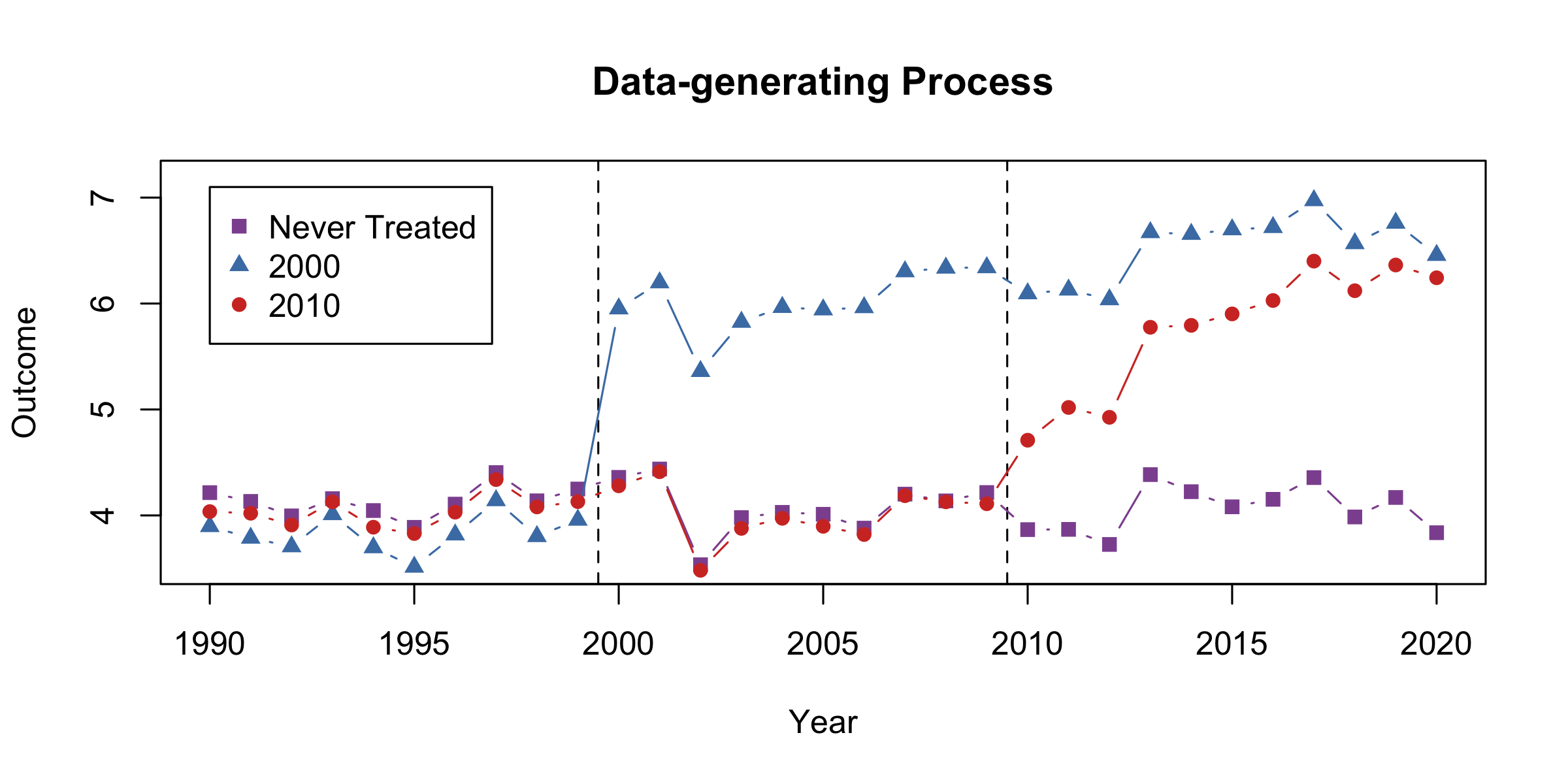
Example data with heterogeneous treatment effects

Estimate Two-stage Difference-in-Differences

First, lets estimate a static did. There are two things to note here. First, note that I can use fixest::feols formula including the | for specifying fixed effects and fixest::i for improved factor variable support. Second, note that did2s returns a fixest estimate object, so fixest::etable, fixest::coefplot, and fixest::iplot all work as expected.

# Static
static <- did2s(
  df_het,
  yname = "dep_var", first_stage = ~ 0 | state + year,
  second_stage = ~ i(treat, ref = FALSE), treatment = "treat",
  cluster_var = "state"
)
#> Running Two-stage Difference-in-Differences
#>  - first stage formula `~ 0 | state + year`
#>  - second stage formula `~ i(treat, ref = FALSE)`
#>  - The indicator variable that denotes when treatment is on is `treat`
#>  - Standard errors will be clustered by `state`

fixest::etable(static)
#>                            static
#> Dependent Var.:           dep_var
#>                                  
#> treat = TRUE    2.152*** (0.0476)
#> _______________ _________________
#> S.E. type                  Custom
#> Observations               46,500
#> R2                        0.33790
#> Adj. R2                   0.33790
#> ---
#> Signif. codes: 0 '***' 0.001 '**' 0.01 '*' 0.05 '.' 0.1 ' ' 1

This is very close to the true treatment effect of ~2.23.

Then, let’s estimate an event study did. Note that relative year has a value of Inf for never treated, so I put this as a reference in the second stage formula.

# Event Study
es <- did2s(df_het,
  yname = "dep_var", first_stage = ~ 0 | state + year,
  second_stage = ~ i(rel_year, ref = Inf), treatment = "treat",
  cluster_var = "state"
)
#> Running Two-stage Difference-in-Differences
#>  - first stage formula `~ 0 | state + year`
#>  - second stage formula `~ i(rel_year, ref = Inf)`
#>  - The indicator variable that denotes when treatment is on is `treat`
#>  - Standard errors will be clustered by `state`

And plot the results:

fixest::iplot(es, main = "Event study: Staggered treatment", xlab = "Relative time to treatment", col = "steelblue", ref.line = -0.5, drop = "Inf")

# Add the (mean) true effects
true_effects <- head(tapply((df_het$te + df_het$te_dynamic), df_het$rel_year, mean), -1)
points(-20:20, true_effects, pch = 20, col = "black")

# Legend
legend(
  x = -20, y = 3, col = c("steelblue", "black"), pch = c(20, 20),
  legend = c("Two-stage estimate", "True effect")
)

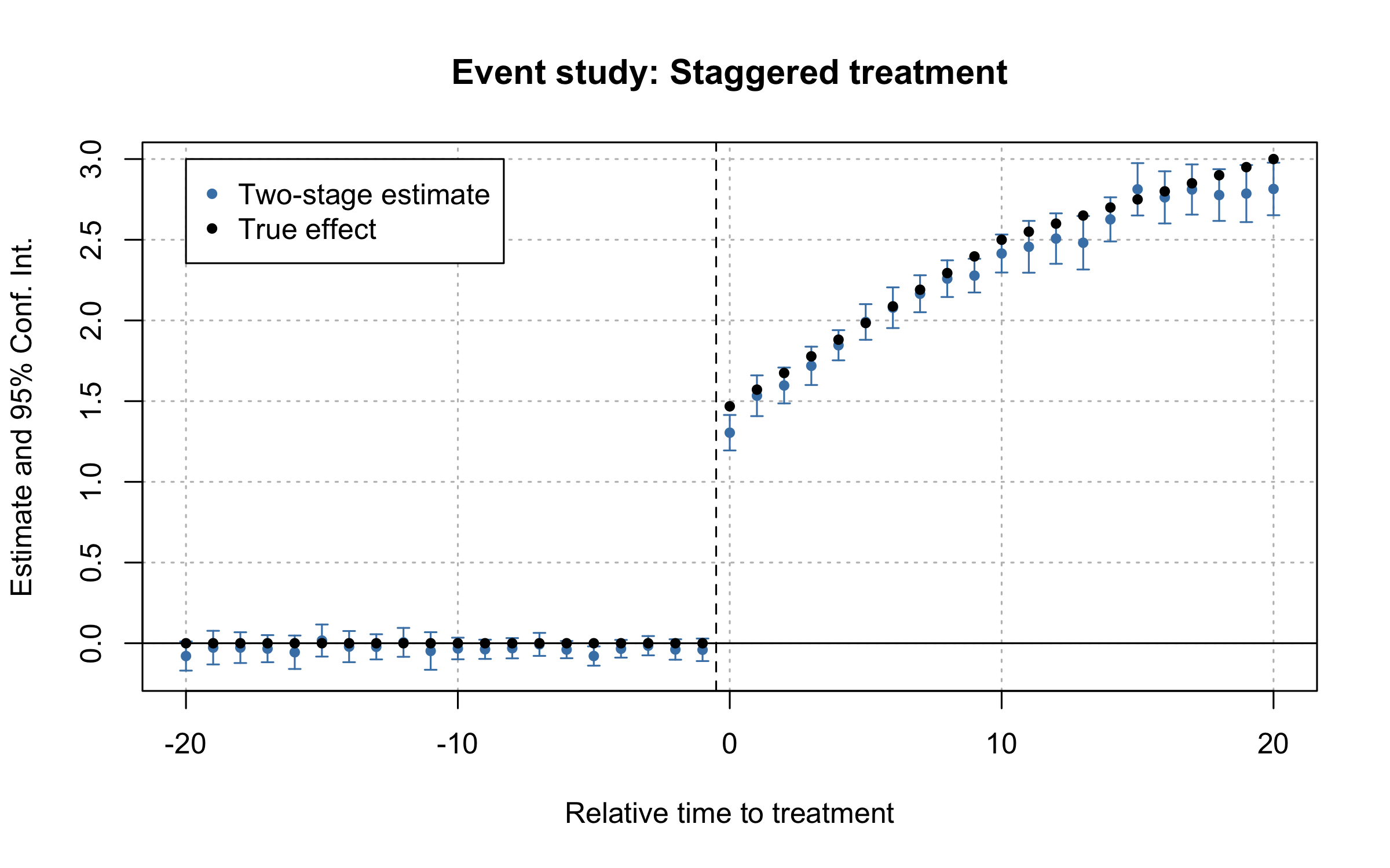
Event-study plot with example data

Comparison to TWFE

twfe <- feols(dep_var ~ i(rel_year, ref = c(Inf, -1)) | unit + year, data = df_het)

fixest::iplot(
  list(es, twfe),
  sep = 0.2, ref.line = -0.5,
  col = c("steelblue", "#82b446"), pt.pch = c(20, 18),
  xlab = "Relative time to treatment",
  main = "Event study: Staggered treatment (comparison)",
  drop = "Inf"
)

# Legend
legend(
  x = -20, y = 3, col = c("steelblue", "#82b446"), pch = c(20, 18),
  legend = c("Two-stage estimate", "TWFE")
)

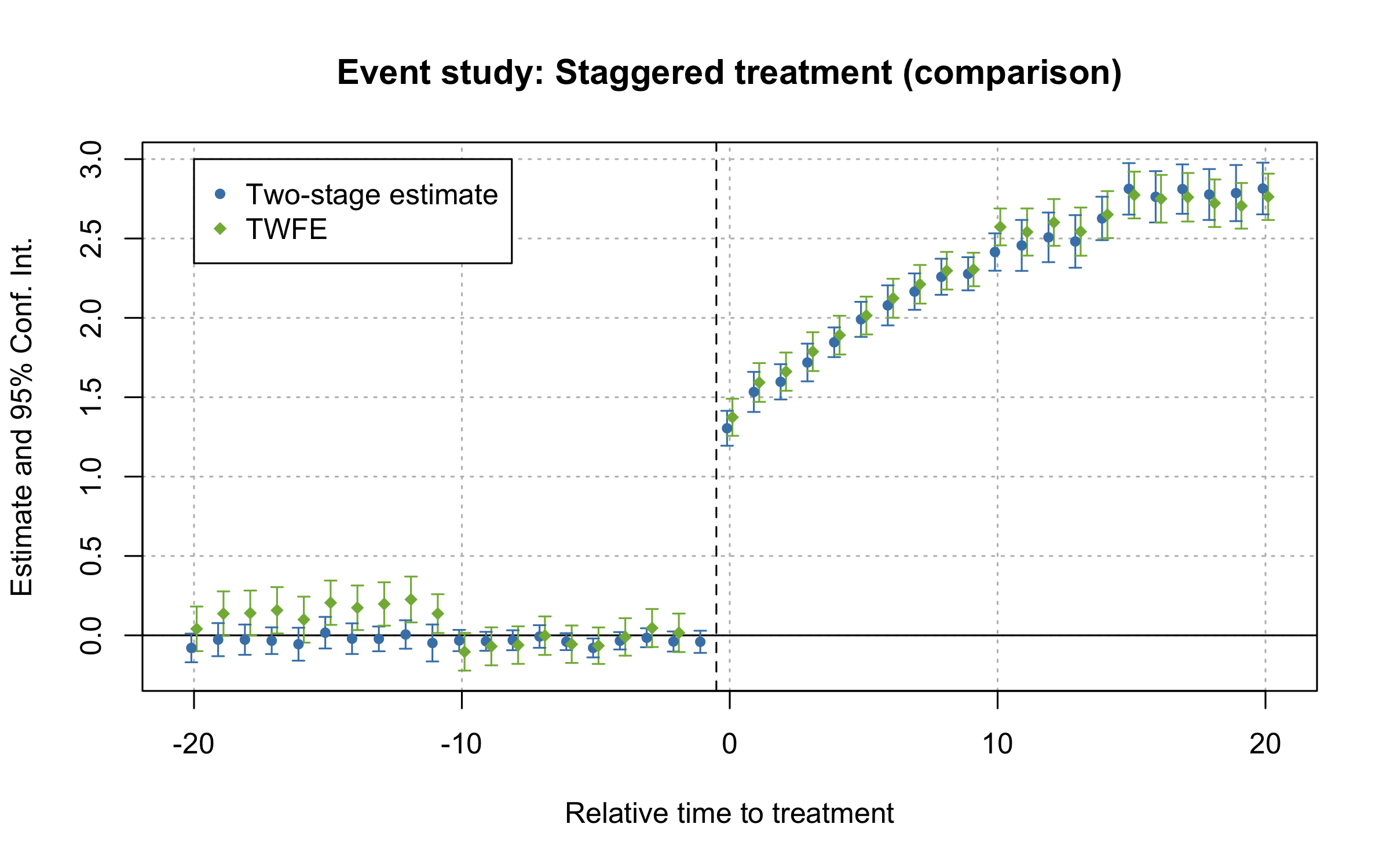
TWFE and Two-Stage estimates of Event-Study

Honest DID

In version 1.1.0, we added support for computing a sensitivity analysis using the approach of Rambachan and Roth (2021).

Here’s an example using data from here. The provided dataset ehec_data.dta contains a state-level panel dataset on health insurance coverage and Medicaid expansion. The variable dins shows the share of low-income childless adults with health insurance in the state. The variable yexp2 gives the year that a state expanded Medicaid coverage under the Affordable Care Act, and is missing if the state never expanded.

library(HonestDiD)
library(ggplot2)

df <- haven::read_dta("https://raw.githubusercontent.com/Mixtape-Sessions/Advanced-DID/main/Exercises/Data/ehec_data.dta")

df$treated <- ifelse(is.na(df$yexp2), 0, 1 * (df$year >= df$yexp2))
df$rel_year <- ifelse(is.na(df$yexp2), -100, df$year - df$yexp2)

# Estimate did2s
es_did2s <- did2s(
  df,
  yname = "dins",
  first_stage = ~ 0 | stfips + year,
  second_stage = ~ 0 + i(rel_year, ref = -100),
  treatment = "treated",
  cluster_var = "stfips"
)
#> Running Two-stage Difference-in-Differences
#>  - first stage formula `~ 0 | stfips + year`
#>  - second stage formula `~ 0 + i(rel_year, ref = -100)`
#>  - The indicator variable that denotes when treatment is on is `treated`
#>  - Standard errors will be clustered by `stfips`

iplot(es_did2s, drop = "-100")

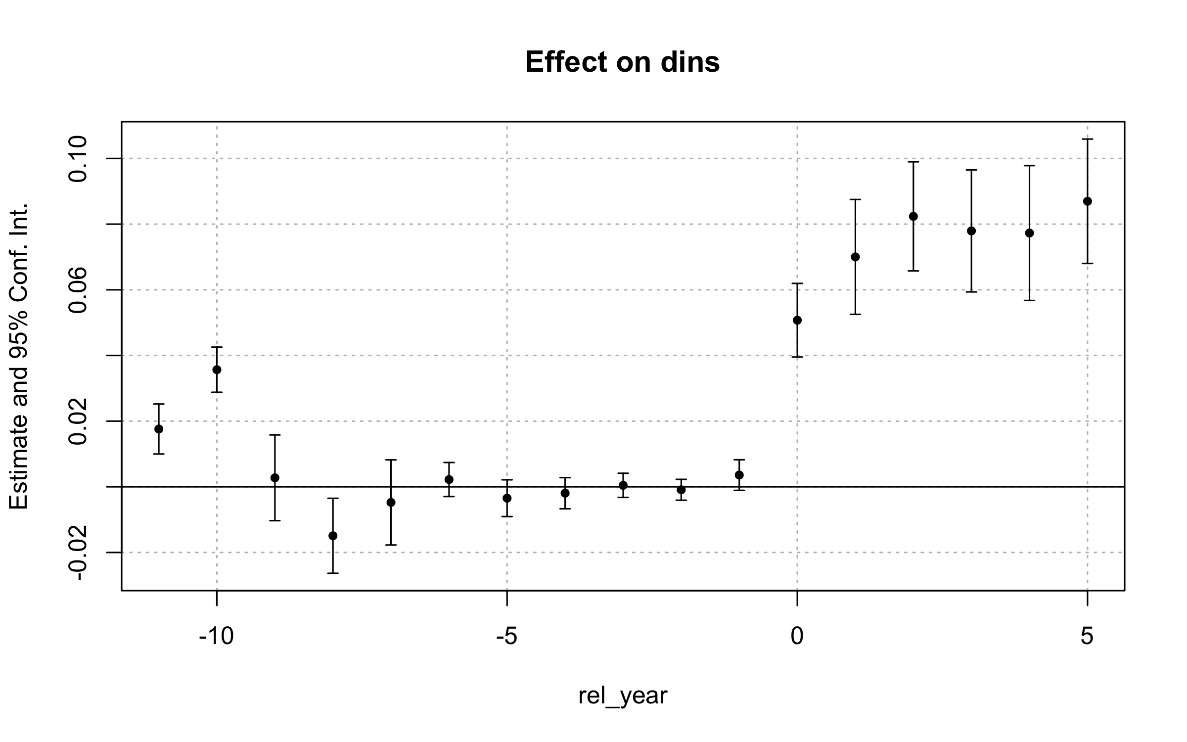
Estimates of the effect of Medicaid expansion on health insurance coverage

# Relative Magnitude sensitivity analysis
sensitivity_results <- es_did2s |> 
  # Take fixest obj and convert for `honest_did_did2s`
  get_honestdid_obj_did2s(coef_name = "rel_year") |>
  # Run sensitivity analysis
  honest_did_did2s(
    e = 0,
    type = "relative_magnitude",
    Mbarvec = seq(from = 0.5, to = 2, by = 0.5)
  )
#> Warning in .ARP_computeCI(betahat = betahat, sigma = sigma, numPrePeriods =
#> numPrePeriods, : CI is open at one of the endpoints; CI length may not be
#> accurate
#> Warning in .ARP_computeCI(betahat = betahat, sigma = sigma, numPrePeriods =
#> numPrePeriods, : CI is open at one of the endpoints; CI length may not be
#> accurate
#> Warning in .ARP_computeCI(betahat = betahat, sigma = sigma, numPrePeriods =
#> numPrePeriods, : CI is open at one of the endpoints; CI length may not be
#> accurate

# Create plot
HonestDiD::createSensitivityPlot_relativeMagnitudes(
  sensitivity_results$robust_ci,
  sensitivity_results$orig_ci
)

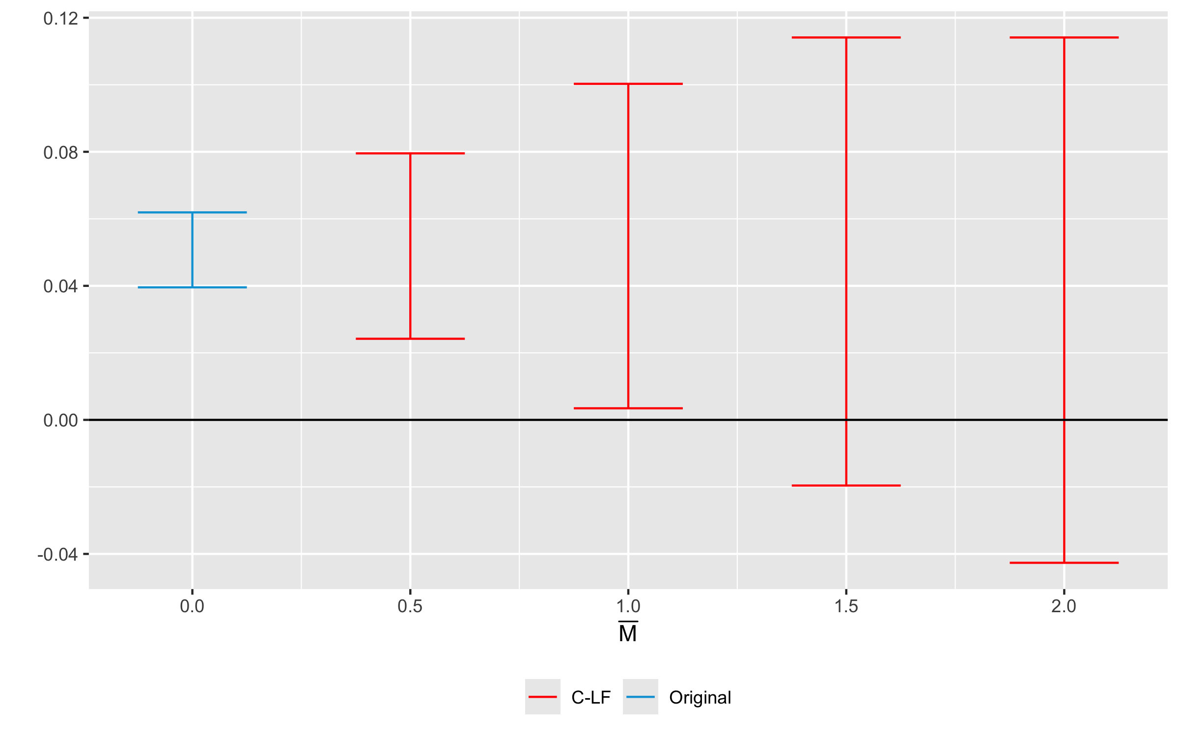
Sensitivity analysis for the example data

Event-study plot

library(tidyverse)
#> ── Attaching core tidyverse packages ──────────────────────── tidyverse 2.0.0 ──
#> ✔ dplyr     1.1.4     ✔ readr     2.1.5
#> ✔ forcats   1.0.0     ✔ stringr   1.5.1
#> ✔ lubridate 1.9.3     ✔ tibble    3.2.1
#> ✔ purrr     1.0.2     ✔ tidyr     1.3.1
#> ── Conflicts ────────────────────────────────────────── tidyverse_conflicts() ──
#> ✖ dplyr::filter() masks stats::filter()
#> ✖ dplyr::lag()    masks stats::lag()
#> ℹ Use the conflicted package (<http://conflicted.r-lib.org/>) to force all conflicts to become errors

data(df_het)
df = df_het
multiple_ests = did2s::event_study(
  data = df |> mutate(g = ifelse(g == Inf, NA, g)) |> as.data.frame(),
  gname = "g",
  idname = "unit",
  tname = "year",
  yname = "dep_var",
  estimator = "all"
)
#> Note these estimators rely on different underlying assumptions. See Table 2 of `https://arxiv.org/abs/2109.05913` for an overview.
#> Estimating TWFE Model
#> Estimating using Gardner (2021)
#> Estimating using Callaway and Sant'Anna (2020)
#> Estimating using Sun and Abraham (2020)
#> Estimating using Borusyak, Jaravel, Spiess (2021)
#> Estimating using Roth and Sant'Anna (2021)

did2s::plot_event_study(multiple_ests)

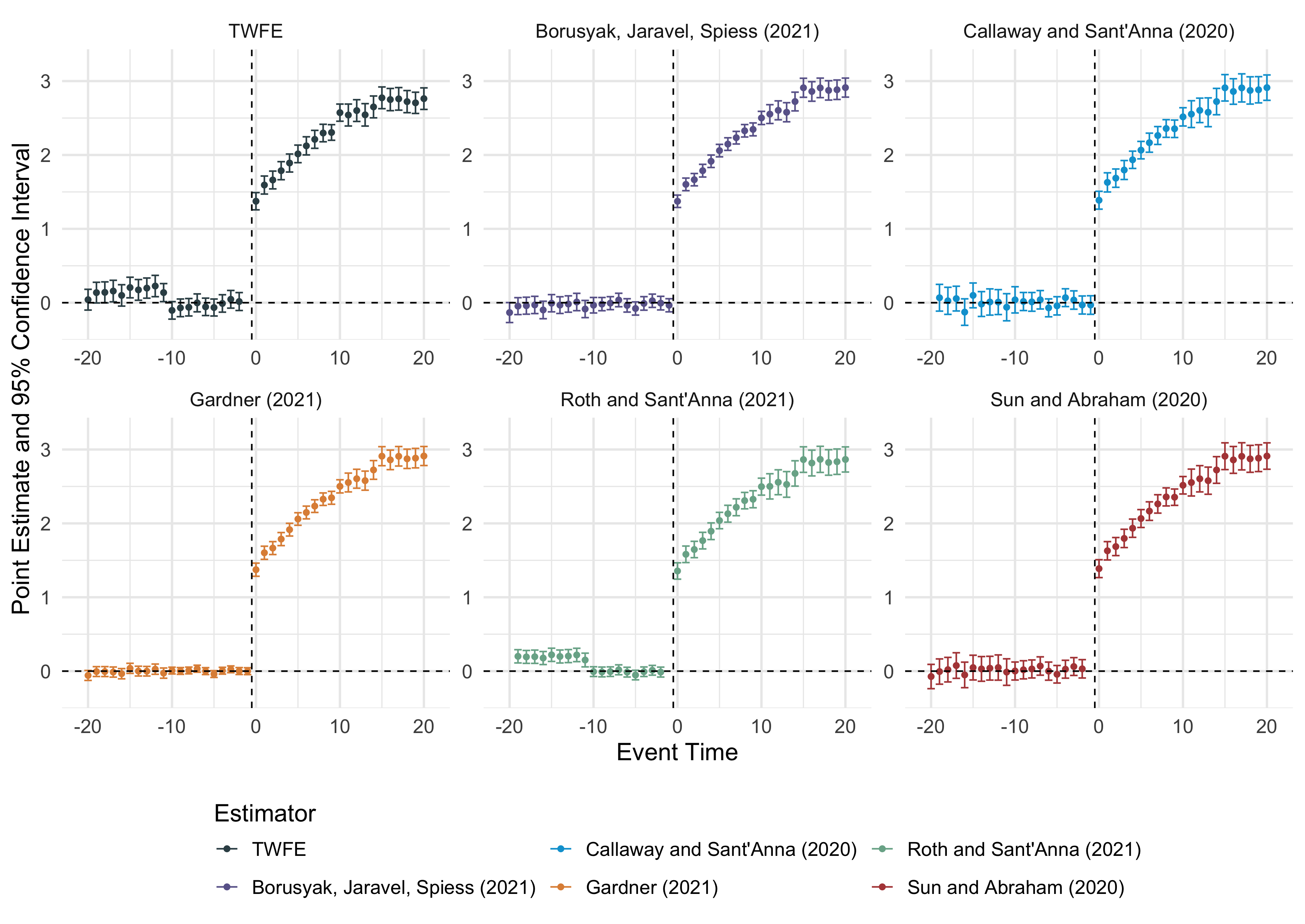
Multiple event-study estimators

Citation

If you use this package to produce scientific or commercial publications, please cite according to:

citation(package = "did2s")
#> To cite did2s in publications use:
#> 
#>   Butts & Gardner, "The R Journal: did2s: Two-Stage
#>   Difference-in-Differences", The R Journal, 2022
#> 
#> A BibTeX entry for LaTeX users is
#> 
#>   @Manual{,
#>     title = {did2s: Two-Stage Difference-in-Differences Following Gardner (2021)},
#>     author = {Kyle Butts and John Gardner},
#>     year = {2021},
#>     url = {https://journal.r-project.org/articles/RJ-2022-048/},
#>   }

References

Gardner, John. 2021. “Two-Stage Difference-in-Differences.” Working Paper. https://jrgcmu.github.io/2sdd_current.pdf.