calibmsm
Calibration Plots for the Transition Probabilities from Multistate Models
Assess the calibration of an existing (i.e. previously developed) multistate
model through calibration plots.
Calibration is assessed using one of three methods. 1) Calibration methods for
binary logistic regression models applied at a fixed time point in conjunction
with inverse probability of censoring weights. 2) Calibration methods for
multinomial logistic regression models applied at a fixed time point in conjunction
with inverse probability of censoring weights. 3) Pseudo-values estimated using
the Aalen-Johansen estimator of observed risk. All methods are applied in conjunction
with landmarking when required. These calibration plots evaluate the calibration
(in a validation cohort of interest) of the transition probabilities estimated from an
existing multistate model. While package development has focused on multistate
models, calibration plots can be produced for any model which utilises information
post baseline to update predictions (e.g. dynamic models); competing risks models;
or standard single outcome survival models, where predictions can be made at
any landmark time. Please see Pate et al. (2024)
calibmsm


The goal of calibmsm is to provide a set of tools for estimating calibration plots when validating an existing (i.e. previously developed) multistate model. While the vignettes and articles for this package focus on assessing the calibration of a multistate model, calibration plots can also be produced for predicted risks from dynamic models, landmark super models, competing risks models and standard single outcome survival models, where predictions can be made at any landmark time.
For a detailed guide on how to use calibmsm please see the Overview vignette.
Installation
The package can be installed from CRAN as follows:
install.packages("calibmsm")
You can install the development version of calibmsm from GitHub with:
# install.packages("devtools")
devtools::install_github("alexpate30/calibmsm")
Example
This is a basic example which shows you how to assess the calibration of
the transition probabilities at 5 years follow up for individuals out of
state j = 1 at time s = 0 using the BLR-IPCW approach. Please see
the Overview vignette for examples of how to assess calibration using
the pseudo-value and MLR-IPCW approaches, as well as details of the
methodology.
The predicted transition probabilities are stored in tps0, the
individuals data are stored in ebmtcal, and the data in msdata
format are stored in msebmtcal. Calibration curves are estimated using
calib_msm using the BLR-IPCW method (calib.type = 'blr') with
inverse probability of censoring weights are calculated based on
variables year, age, prophylaxis and donor gender match. The
calibration curves are estimated using restricted cubic splines with 3
knots. A 95% confidence interval is calculated using bootstrapping with
200 bootstrap replicates.
## Load calibmsm
library(calibmsm)

## Extract relevant predicted risks from tps0
tp_pred_s0 <- dplyr::select(dplyr::filter(tps0, j == 1), any_of(paste("pstate", 1:6, sep = "")))

## Calculate observed event probabilities
dat_calib_blr <-
  calib_msm(data_ms = msebmtcal,
            data_raw = ebmtcal,
            j = 1,
            s = 0,
            t = 1826,
            tp_pred = tp_pred_s0,
            calib_type = "blr",
            curve_type = "rcs",
            rcs_nk = 3,
            w_covs = c("year", "agecl", "proph", "match"),
            CI = 95,
            CI_R_boot = 200)
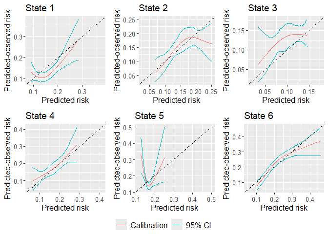
We can then plot the calibration plots:
plot(dat_calib_blr, combine = TRUE, nrow = 2, ncol = 3, axis.titles.x = c(4,5,6), axis.titles.y = c(1,4), marg_density = FALSE)
If wanting to include marginal density plots (recommended, also the default) then the output is a gTable, that must then in turn be plotted, i.e:
marg_density_plot <- plot(dat_calib_blr, combine = TRUE, nrow = 2, ncol = 3, axis.titles.x = c(4,5,6), axis.titles.y = c(1,4))
plot(marg_density_plot)
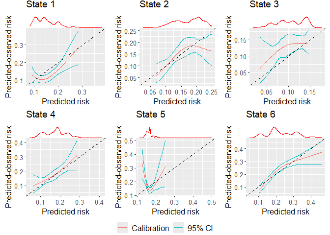
At this step plot can also be replcaed by grid::grid.draw.
Getting help
If you encounter a bug, please file an issue with a minimal reproducible example on GitHub.