Bayesian Weighted Sums

An interface to the Bayesian Weighted Sums model implemented in 'RStan'. It estimates the summed effect of multiple, often moderately to highly correlated, continuous predictors. Its applications can be found in analysis of exposure mixtures. The model was proposed by Hamra, Maclehose, Croen, Kauffman, and Newschaffer (2021) . This implementation includes an extension to model binary outcome.

bws

The goal of bws is to provide a user-friendly and efficient implementation of the Bayesian Weighted Sums (BWS) described by Hamra, Maclehose, Croen, Kauffman, and Newschaffer (2021) with some extensions to work with binary and count response data.

Installation

You can install the development version from GitHub with:

# install.packages("devtools")
devtools::install_github("phuchonguyen/bws")

Example

This is a basic example which shows you how to fit BWS:

## We first need to simulate some data
set.seed(123)
N <- 100
P <- 3
K <- 2
X <- matrix(rnorm(N*P), N, P)
Z <- matrix(rnorm(N*K), N, K)  # confounders
w <- c(0.3, 0.2, 0.5)
theta0 <- 2
theta1 <- 3
beta <- runif(K, 0.5, 1.5)
y <- theta0 + theta1*theta1*(X%*%w) + Z%*%beta + rnorm(N)
## Fitting BWS is simple
fit <- bws::bws(iter = 2000, y = y, X = X, Z = Z,
         # additional arguments for rstan::sampling
         chains = 4, cores = 2, show_messages = FALSE)
#> Warning: replacing previous import 'lifecycle::last_warnings' by
#> 'rlang::last_warnings' when loading 'tibble'
#> Warning: replacing previous import 'lifecycle::last_warnings' by
#> 'rlang::last_warnings' when loading 'pillar'

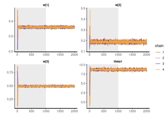
Since the implementation uses Stan and returns an rstanfit object, users can enjoy all the functionalities provided in rstan to analyze the fitted model:

rstan::traceplot(fit, pars = c("w", "theta1"), inc_warmup = TRUE, nrow = 2)

print(fit, pars = c("w", "theta1"))
#> Inference for Stan model: bws.
#> 4 chains, each with iter=2000; warmup=1000; thin=1; 
#> post-warmup draws per chain=1000, total post-warmup draws=4000.
#> 
#>        mean se_mean   sd 2.5%  25%  50%  75% 97.5% n_eff Rhat
#> w[1]   0.32       0 0.01 0.30 0.31 0.32 0.33  0.34  5292    1
#> w[2]   0.19       0 0.01 0.17 0.18 0.19 0.19  0.21  5750    1
#> w[3]   0.49       0 0.01 0.47 0.49 0.49 0.50  0.51  6125    1
#> theta1 8.71       0 0.19 8.34 8.59 8.71 8.84  9.08  5388    1
#> 
#> Samples were drawn using NUTS(diag_e) at Mon Jun 13 00:06:38 2022.
#> For each parameter, n_eff is a crude measure of effective sample size,
#> and Rhat is the potential scale reduction factor on split chains (at 
#> convergence, Rhat=1).
rstan::plot(fit)
#> ci_level: 0.8 (80% intervals)
#> outer_level: 0.95 (95% intervals)

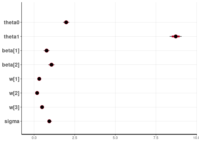
The model inferred the correct weights, which are set to 0.3, 0.2, 0.5 in the simulation.

Reference:

Hamra, G.B.; Maclehose, R.F.; Croen, L.; Kauffman, E.M.; Newschaffer, C. Bayesian Weighted Sums: A Flexible Approach to Estimate Summed Mixture Effects. International Journal of Environmental Research and Public Health 2021, 18, 1373. link