badp
Bayesian Averaging for Dynamic Panels
Implements Bayesian model averaging for dynamic panels with weakly
exogenous regressors as described in the paper by
Moral-Benito (2013,
badp: Bayesian Averaging for Dynamic Panels
badp: Bayesian Averaging for Dynamic Panels 


Overview
The badp package implements Bayesian model averaging (BMA) for dynamic panels with weakly exogenous regressors, following the methodology of Moral-Benito (2016). This addresses both:
- Model uncertainty (selecting among many candidate regressors),
- Reverse causality (weak exogeneity, which permits current values of regressors to correlate with past shocks and other regressors).
The package features:
- Tools to estimate the entire model space (via maximum likelihood) and calculate Bayesian information criterion (BIC) for each variant.
- Flexible model priors (binomial, binomial-beta, optional dilution prior).
- A selectable learning rate for the model weights (
weightingandetainbma()), so the sensitivity of a conclusion to the marginal likelihood approximation can be checked without re-estimating the model space. - Comprehensive BMA statistics, including posterior inclusion probabilities (PIPs), posterior means, and posterior standard deviations (regular or robust).
- Functions to visualize prior and posterior model probabilities.
- Jointness measures for pairs of regressors, indicating whether they are complements or substitutes.
- Support for parallel computing to handle large model spaces.
Installation
You can install the released version of badp from CRAN with:
install.packages("badp")
And the development version from GitHub with:
# install.packages("devtools")
devtools::install_github("badp-project/badp")
Once installed, simply load the package:
library(badp)
Getting Started
Data Preparation
Your data should be in the following format:
- A time column (e.g.,
year), - An entity column (e.g.,
country), - A dependent variable column (the variable of interest,
e.g.
gdp), - Remaining columns as potential regressors.
A convenience function join_lagged_col() can help transform a dataset
that already contains both a variable and its lagged version into the
required format.
You can also use feature_standardization() to perform mean-centering,
demeaning (entity/time effects), or scaling (standardization) as needed.
For example:
library(magrittr)

set.seed(20)

# Features are scaled and demeaned,
# then centralized around the mean within cross-sections (fixed time effects)
data_prepared <- badp::economic_growth[, 1:5] %>%
  badp::feature_standardization(
    excluded_cols = c(country, year, gdp)
  ) %>%
  badp::feature_standardization(
    group_by_col  = year,
    excluded_cols = country,
    scale         = FALSE
  )
Estimating the Model Space
The function optim_model_space() estimates all possible models (each
possible subset of regressors) via maximum likelihood, returning an
object of class badp_model_space.
Note: with strongly correlated regressors, both the estimation and
the subsequent statistics step may emit warnings (e.g. NaNs produced,
or a message that some models did not converge). The exact reason is
non-trivial: it is typically connected to degenerate behavior of the
likelihood function for some of the models, and understanding it for a
particular dataset requires inspecting the data (e.g. correlations
between regressors), the behavior of the likelihood, and the per-model
per-model diagnostics returned by convergence(). A good starting point
is to check which models are affected and how much posterior model
probability they carry - if it is negligible, the warnings can usually
be treated as expected behavior.
For small to moderately sized datasets:
model_space <- badp::optim_model_space(
  df             = data_prepared,
  dep_var_col    = gdp,
  timestamp_col  = year,
  entity_col     = country,
  init_value     = function(n) runif(n, -10, 10)
)
For larger datasets, you can leverage multiple cores:
library(parallel)

# Choose an appropriate number of cores, taking into account system-level limits
cores <- as.integer(Sys.getenv("_R_CHECK_LIMIT_CORES_", unset = NA))
if (is.na(cores)) {
  cores <- detectCores()
} else {
  cores <- min(cores, detectCores())
}
cl <- makeCluster(cores)

model_space <- badp::optim_model_space(
  df             = data_prepared,
  timestamp_col  = year,
  entity_col     = country,
  dep_var_col    = gdp,
  init_value     = function(n) runif(n, -10, 10),
  cl             = cl
)

stopCluster(cl)
A progress bar is displayed to easily track the ongoing computation.
Performing Bayesian Model Averaging
After preparing the model space, run bma() to obtain posterior model
probabilities, posterior inclusion probabilities (PIPs), and other BMA
statistics under the binomial and binomial-beta model priors:
bma_results <- badp::bma(model_space, round = 3)

# BMA statistics under each model prior
badp::bma_table(bma_results)
#>           PIP     PM   PSD  PSDR  PMcon PSDcon PSDRcon %(+)
#> gdp_lag    NA  1.078 0.110 0.227  1.078  0.110   0.227  100
#> ish     0.710  0.085 0.061 0.090  0.120  0.032   0.085  100
#> sed     0.714 -0.046 0.061 0.111 -0.065  0.064   0.127    0
badp::bma_table(bma_results, prior = "beta")
#>           PIP     PM   PSD  PSDR  PMcon PSDcon PSDRcon %(+)
#> gdp_lag    NA  1.078 0.109 0.238  1.078  0.109   0.238  100
#> ish     0.765  0.091 0.058 0.090  0.119  0.033   0.085  100
#> sed     0.768 -0.048 0.062 0.114 -0.063  0.064   0.126    0

# Posterior inclusion probabilities on their own
sort(badp::pip(bma_results), decreasing = TRUE)
#>   sed   ish
#> 0.714 0.710

# Prior and posterior model sizes
badp::model_size_table(bma_results)
#>               Prior model size Posterior model size
#> Binomial                     1                1.424
#> Binomial-beta                1                1.533
Key columns in the BMA output include: - PIP: Posterior inclusion probability for each regressor. - PM: Posterior mean of each parameter (averaged over all models). - PSD/PSDR: Posterior standard deviations (regular/robust) of each parameter - %(+): Percentage of models (among those that include a given regressor) in which the parameter estimate is positive.
Visualizing Prior and Posterior Probabilities
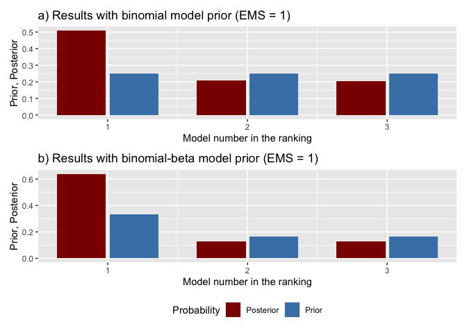
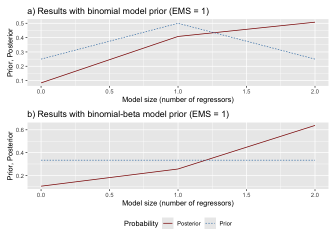
model_pmp(): Shows prior vs. posterior model probabilities, ranking models from best to worst.model_sizes(): Displays how prior vs. posterior probabilities mass is distributed across different model sizes.
# Prior vs. posterior model probabilities, three best models.
# `type = "histogram"` draws bars, which read well for a handful of models;
# the default `"line"` is better once there are many.
badp::model_pmp(bma_results, top = 3, type = "histogram")
# Probabilities by model size
badp::model_sizes(bma_results)
Selecting the Best Models
Use best_models() to extract specific information about the top-ranked
models:
# Retrieve the 5 best models according to binomial prior
top3_binom <- badp::best_models(bma_results, prior = "binomial", best = 3)

# Which regressors enter each of the three models
top3_binom
#> Best 3 of 4 models, ranked by the binomial posterior model probability
#>
#>         No. 1 No. 2 No. 3
#> gdp_lag x     x     x
#> ish     x     .     x
#> sed     x     x     .
#> PMP     0.508 0.206 0.202
#>
#> 'x' marks an included regressor. Use summary() for the estimates,
#> plot() for the same tables as a graphic, and [[i]] for one model.

# Estimates for all three, with robust standard errors
summary(top3_binom, robust = TRUE)
#> Best Models Summary
#> ===================
#>
#> Models shown:            3 of 4
#> Ranking model prior:     binomial
#> Posterior mass covered:  0.916
#> Regressors per model:    2, 1, 1
#>
#> Estimates (robust standard errors in parentheses):
#>         No. 1            No. 2            No. 3
#> gdp_lag 1.079 (0.273)*** 1.126 (0.151)*** 1.027 (0.191)***
#> ish     0.119 (0.086)                     0.121 (0.082)
#> sed     -0.06 (0.126)    -0.077 (0.127)
#> PMP     0.508            0.206            0.202
#>
#> Signif. codes: 0.01 '***'  0.05 '**'  0.1 '*'

# A single model on its own
top3_binom[[1]]
#> Model No. 1 of the binomial ranking
#> Posterior model probability: 0.508
#> Log-likelihood: -35.154 (df = 29)
#> Regressors included: ish, sed
#>
#>         Estimate Std. Error Pr(>|z|)
#> gdp_lag    1.079      0.111    0.000 ***
#> ish        0.119      0.033    0.000 ***
#> sed       -0.060      0.063    0.342
#>
#> Standard errors: conventional. Wald p-values, standard normal reference.
#> Signif. codes: 0.01 '***'  0.05 '**'  0.1 '*'
Jointness Measures
Assess whether two regressors tend to co-occur (complements) or exclude
each other (substitutes) using jointness(). By default, it calculates
the Hofmarcher et al. (2018) measure:
joint_measures <- badp::jointness(bma_results)
head(joint_measures)
#>       ish   sed
#> ish    NA 0.159
#> sed 0.505    NA
You can also specify older measures, such as "LS" (Ley & Steel) or
"DW" (Doppelhofer & Weeks):
joint_measures_ls <- badp::jointness(bma_results, measure = "LS")
Example
Below is a minimal reproducible workflow:
# 1) Data preparation
data_prepared <- badp::economic_growth[, 1:5] %>%
  badp::feature_standardization(
    excluded_cols = c(country, year, gdp)
  ) %>%
  badp::feature_standardization(
    group_by_col  = year,
    excluded_cols = country,
    scale         = FALSE
  )

# 2) Estimate model space
model_space <- badp::optim_model_space(
  df            = data_prepared,
  dep_var_col   = gdp,
  timestamp_col = year,
  entity_col    = country,
  init_value    = function(n) rep(0.5, n),
)

# 3) Run Bayesian Model Averaging
bma_obj <- badp::bma(
  model_space = model_space
)

# 4) Inspect the top 3 models under binomial prior
best_3 <- badp::best_models(
  x = bma_obj,
  prior = "binomial",
  best = 3
)
best_3                      # inclusion table for the three models
#> Best 3 of 4 models, ranked by the binomial posterior model probability
#>
#>         No. 1 No. 2 No. 3
#> gdp_lag x     x     x
#> ish     x     .     x
#> sed     x     x     .
#> PMP     0.508 0.206 0.202
#>
#> 'x' marks an included regressor. Use summary() for the estimates,
#> plot() for the same tables as a graphic, and [[i]] for one model.
coef(best_3[[1]], se = TRUE)  # estimates for the best one
#>            Estimate Std. Error Robust Std. Error     Pr(>|z|) Robust Pr(>|z|)
#> gdp_lag  1.07934984 0.11099769        0.27305145 2.380587e-22    7.720409e-05
#> ish      0.11929274 0.03293347        0.08553459 2.920699e-04    1.631146e-01
#> sed     -0.06010157 0.06326577        0.12591614 3.421196e-01    6.331384e-01
Troubleshooting
- Cannot install required packages / setup renv environment
Make sure to go through the displayed errors. The problem might be connected to your OS environment. E.g. you might see an information like the following:
Configuration failed to find one of freetype2 libpng libtiff-4 libjpeg. Try installing:
 * deb: libfreetype6-dev libpng-dev libtiff5-dev libjpeg-dev (Debian, Ubuntu, etc)
 * rpm: freetype-devel libpng-devel libtiff-devel libjpeg-devel (Fedora, CentOS, RHEL)
 * csw: libfreetype_dev libpng16_dev libtiff_dev libjpeg_dev (Solaris)
In such case you should first try installing the recommended packages. With properly configured system environment everything should work fine.
References
- Moral-Benito, E. (2016). “Growth Empirics in Panel Data Under Model Uncertainty and Weak Exogeneity.” Journal of Applied Econometrics.
- Ley, E. and Steel, M. F. J. (2007). “Jointness in Bayesian Variable Selection with Applications to Growth Regression.” Journal of Macroeconomics.
- Doppelhofer, G. and Weeks, M. (2009). “Jointness of Growth Determinants.” Journal of Applied Econometrics.
- Hofmarcher, P., Crespo Cuaresma, J., Grün, B., Humer, S., and Moser, M. (2018). “Bivariate jointness measures in Bayesian Model Averaging: Solving the conundrum.” Journal of Macroeconomics.
(Additional references related to the methodology can be found in the package vignette.)
Contributions and Issues
We welcome bug reports, feature requests, and contributions. Feel free to open an issue or pull request on GitHub.
License
This package is distributed under the MIT license. See the LICENSE file for details.