Distributions Compatible with Automatic Differentiation by 'RTMB'

Extends the functionality of the 'RTMB' < https://kaskr.r-universe.dev/RTMB> package by providing a collection of non-standard probability distributions compatible with automatic differentiation (AD). While 'RTMB' enables flexible and efficient modelling, including random effects, its built-in support is limited to standard distributions. The package adds additional AD-compatible distributions, broadening the range of models that can be implemented and estimated using 'RTMB'. Automatic differentiation and Laplace approximation are described in Kristensen et al. (2016) .

RTMBdist — AD distribution library

The RTMB package enables powerful and flexible statistical modelling with rich random effect structures using automatic differentiation (AD). However, its built-in support for probability distributions is limited to standard cases. RTMBdist fills this gap by providing a collection of non-standard, AD-compatible distributions, extending the range of models that can be implemented and estimated with RTMB. Most of the distributions implemented in RTMBdist allow for automatic simulation and residual calculation by RTMB.

The full list of distributions currently available is given in the List of distributions vignette. There are also a couple of Worked examples demonstrating how to use RTMBdist in practice.

Note that some famous non-standard distributions (Tweedie, SHASHo, COM-Pois, Cauchy) are already implemented in RTMB; check the distributions listed here.

Feel free to contribute a distribution (Guide to adding a distribution) or open an issue!

Installation

You can install the released version from CRAN with:

install.packages("RTMBdist")

or the development version from GitHub with:

remotes::install_github("janolefi/RTMBdist")

Introductory example

library(RTMBdist)

Let’s do numerical maximum likelihood estimation with a gumbel distribution:

# simulate data
x <- rgumbel(100, location = 5, scale = 2)

# negative log-likelihood function
nll <- function(par) {
  x <- OBS(x) # mark x as the response
  loc <- par[1]; ADREPORT(loc)
  scale <- exp(par[2]); ADREPORT(scale)
  -sum(dgumbel(x, loc, scale, log = TRUE))
}

# RTMB AD object
obj <- MakeADFun(nll, c(5, log(2)), silent = TRUE)

# model fitting using AD gradient
opt <- nlminb(obj$par, obj$fn, obj$gr)

# model summary
summary(sdreport(obj))[3:4,]
#>       Estimate Std. Error
#> loc   5.001543  0.2065935
#> scale 1.960676  0.1502500

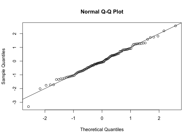
Through the magic of RTMB, we can also immediately simulate new data from the fitted model and calculate residuals:

# simulate new data
x_new <- obj$simulate()$x

# calculate residuals
osa <- oneStepPredict(obj, method = "cdf", trace = FALSE)
qqnorm(osa$res); abline(0, 1)