Tidy Analysis Tools for Mortality, Fertility, Migration and Population Data

Analysing vital statistics based on tools consistent with the tidyverse. Tools are provided for data visualization, life table calculations, computing net migration numbers, Lee-Carter modelling; functional data modelling and forecasting.

vital

The goal of vital is to allow analysis of demographic data using tidy tools.

Installation

You can install the stable version from CRAN:

pak::pak("vital")

You can install the development version from GitHub:

pak::pak("robjhyndman/vital")

Examples

First load the necessary packages.

library(vital)
library(tsibble)
library(dplyr)
library(ggplot2)

vital objects

The basic data object is a vital, which is time-indexed tibble that contains vital statistics such as births, deaths, population counts, and mortality and fertility rates.

Here is an example of a vital object containing mortality data for Norway, with the upper ages collapsed into a final age group of 100+.

norway_mortality <- norway_mortality |>
  collapse_ages(max_age = 100)
norway_mortality
#> # A vital: 37,572 x 7 [1Y]
#> # Key:     Age x Sex [101 x 3]
#>     Year   Age OpenInterval Sex    Population Deaths Mortality
#>    <int> <int> <lgl>        <chr>       <dbl>  <dbl>     <dbl>
#>  1  1900     0 FALSE        Female      30070 2376.    0.0778
#>  2  1900     1 FALSE        Female      28960  842     0.0290
#>  3  1900     2 FALSE        Female      28043  348     0.0123
#>  4  1900     3 FALSE        Female      27019  216.    0.00786
#>  5  1900     4 FALSE        Female      26854  168.    0.00624
#>  6  1900     5 FALSE        Female      25569  140.    0.00538
#>  7  1900     6 FALSE        Female      25534  108.    0.00422
#>  8  1900     7 FALSE        Female      24314   93.5   0.00376
#>  9  1900     8 FALSE        Female      24979   93.5   0.00380
#> 10  1900     9 FALSE        Female      24428   90     0.00365
#> # ℹ 37,562 more rows

We can use functions to see which variables are index, key or vital:

index_var(norway_mortality)
#> [1] "Year"
key_vars(norway_mortality)
#> [1] "Age" "Sex"
vital_vars(norway_mortality)
#>          age          sex       deaths   population
#>        "Age"        "Sex"     "Deaths" "Population"

Plots

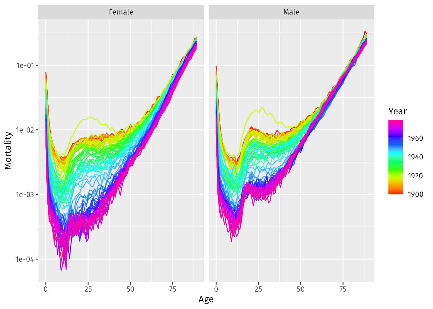
norway_mortality |>
  filter(Sex != "Total", Year < 1980, Age < 90) |>
  autoplot(Mortality) + scale_y_log10()

Life tables and life expectancy

# Life table for Norwegian males in 2000
norway_mortality |>
  filter(Sex == "Male", Year == 2000) |>
  life_table()
#> # A vital: 101 x 13 [?]
#> # Key:     Age x Sex [101 x 1]
#>     Year   Age Sex         mx        qx    lx        dx    Lx    Tx    ex    rx    nx     ax
#>    <int> <int> <chr>    <dbl>     <dbl> <dbl>     <dbl> <dbl> <dbl> <dbl> <dbl> <dbl>  <dbl>
#>  1  2000     0 Male  0.00426  0.00424   1     0.00424   0.996  76.0  76.0 0.996     1 0.0564
#>  2  2000     1 Male  0.000593 0.000593  0.996 0.000590  0.995  75.0  75.3 0.999     1 0.5
#>  3  2000     2 Male  0.000229 0.000229  0.995 0.000228  0.995  74.0  74.3 1.000     1 0.5
#>  4  2000     3 Male  0.000157 0.000157  0.995 0.000156  0.995  73.0  73.3 1.000     1 0.5
#>  5  2000     4 Male  0.000221 0.000221  0.995 0.000220  0.995  72.0  72.3 1.000     1 0.5
#>  6  2000     5 Male  0.000189 0.000189  0.995 0.000188  0.994  71.0  71.4 1.000     1 0.5
#>  7  2000     6 Male  0.000128 0.000128  0.994 0.000127  0.994  70.0  70.4 1.000     1 0.5
#>  8  2000     7 Male  0.000127 0.000127  0.994 0.000126  0.994  69.0  69.4 1.000     1 0.5
#>  9  2000     8 Male  0.000094 0.0000940 0.994 0.0000934 0.994  68.0  68.4 1.000     1 0.5
#> 10  2000     9 Male  0.000217 0.000217  0.994 0.000216  0.994  67.0  67.4 1.000     1 0.5
#> # ℹ 91 more rows

# Life expectancy
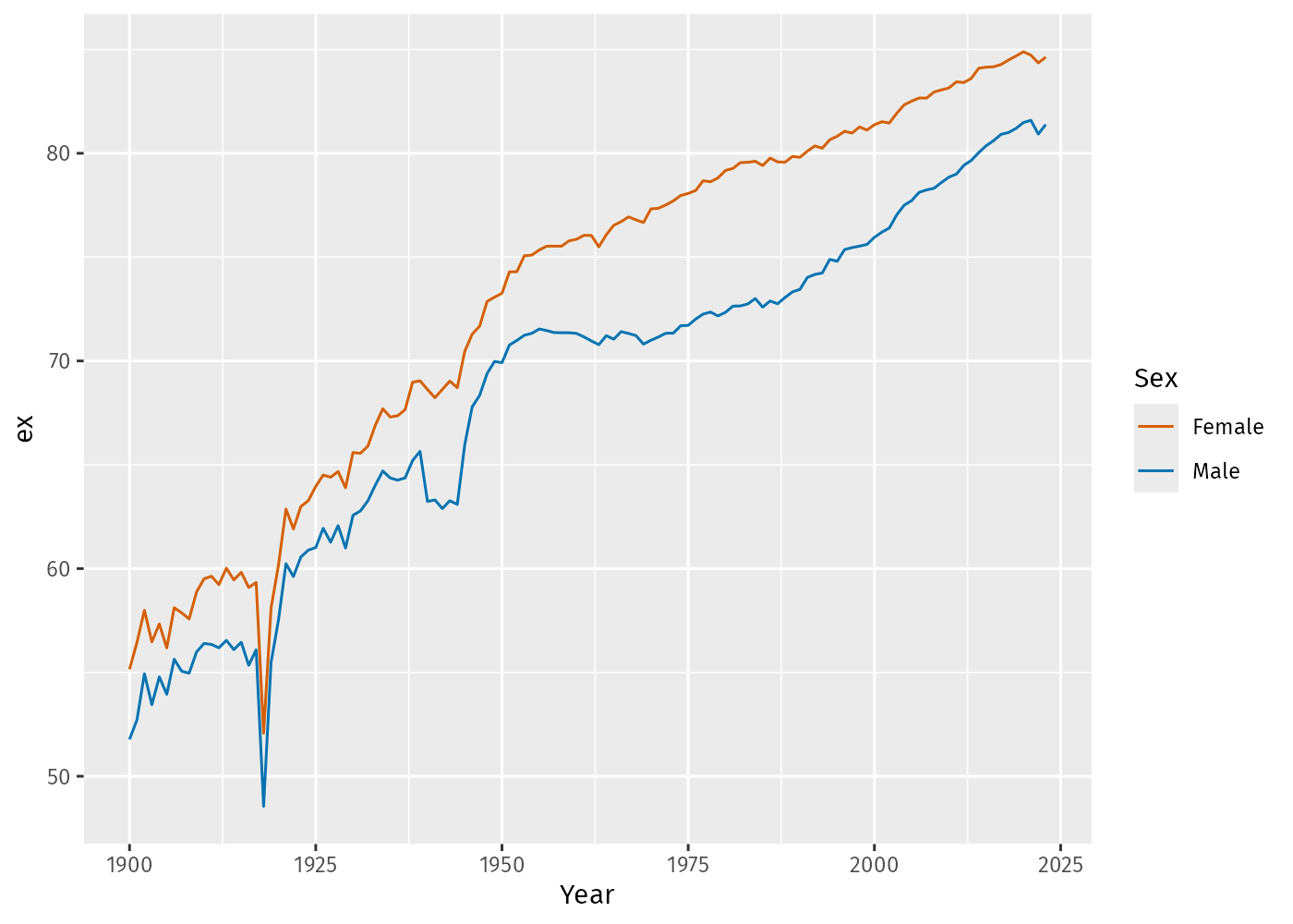
norway_mortality |>
  filter(Sex != "Total") |>
  life_expectancy() |>
  ggplot(aes(x = Year, y = ex, color = Sex)) +
  geom_line()

Smoothing

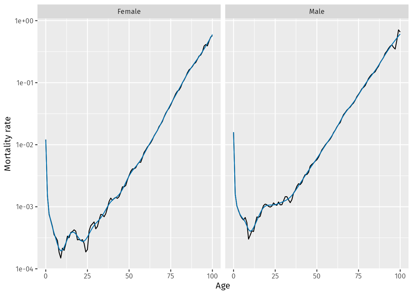
Several smoothing functions are provided: smooth_spline(), smooth_mortality(), smooth_fertility(), and smooth_loess(), each smoothing across the age variable for each year. The smooth_mortality_law() function fits a parametric mortality law instead.

# Smoothed data
norway_mortality |>
  filter(Sex != "Total", Year == 1967) |>
  smooth_mortality(Mortality) |>
  autoplot(Mortality) +
  geom_line(aes(y = .smooth), col = "#0072B2") +
  ylab("Mortality rate") +
  scale_y_log10()

Mortality models

Several mortality models are available including variations on Lee-Carter models (Lee & Carter, JASA, 1992), functional data models (Hyndman & Ullah, CSDA, 2007), generalized age-period-cohort models from the StMoMo package (LC2(), CBD(), APC(), RH(), M7(), PLAT() and GAPC()), and the benchmark models FMEAN() and FNAIVE().

fit <- norway_mortality |>
  filter(Sex != "Total") |>
  model(
    lee_carter = LC(log(Mortality)),
    fdm = FDM(log(Mortality))
  )
fit
#> # A mable: 2 x 3
#> # Key:     Sex [2]
#>   Sex    lee_carter     fdm
#>   <chr>     <model> <model>
#> 1 Female       <LC>   <FDM>
#> 2 Male         <LC>   <FDM>

Models are fitted for all combinations of key variables excluding age.

fit |>
  select(lee_carter) |>
  filter(Sex == "Female") |>
  report()
#> Series: Mortality
#> Model: LC
#> Transformation: log(Mortality)
#>
#> Options:
#>   Adjust method: dt
#>   Jump choice: fit
#>
#> Age functions
#> # A tibble: 101 × 3
#>     Age    ax     bx
#>   <int> <dbl>  <dbl>
#> 1     0 -4.33 0.0151
#> 2     1 -6.16 0.0218
#> 3     2 -6.88 0.0197
#> 4     3 -7.20 0.0190
#> 5     4 -7.35 0.0177
#> # ℹ 96 more rows
#>
#> Time coefficients
#> # A tsibble: 124 x 2 [1Y]
#>    Year    kt
#>   <int> <dbl>
#> 1  1900  118.
#> 2  1901  112.
#> 3  1902  105.
#> 4  1903  111.
#> 5  1904  109.
#> # ℹ 119 more rows
#>
#> Time series model: RW w/ drift
#>
#> Variance explained: 92.39%

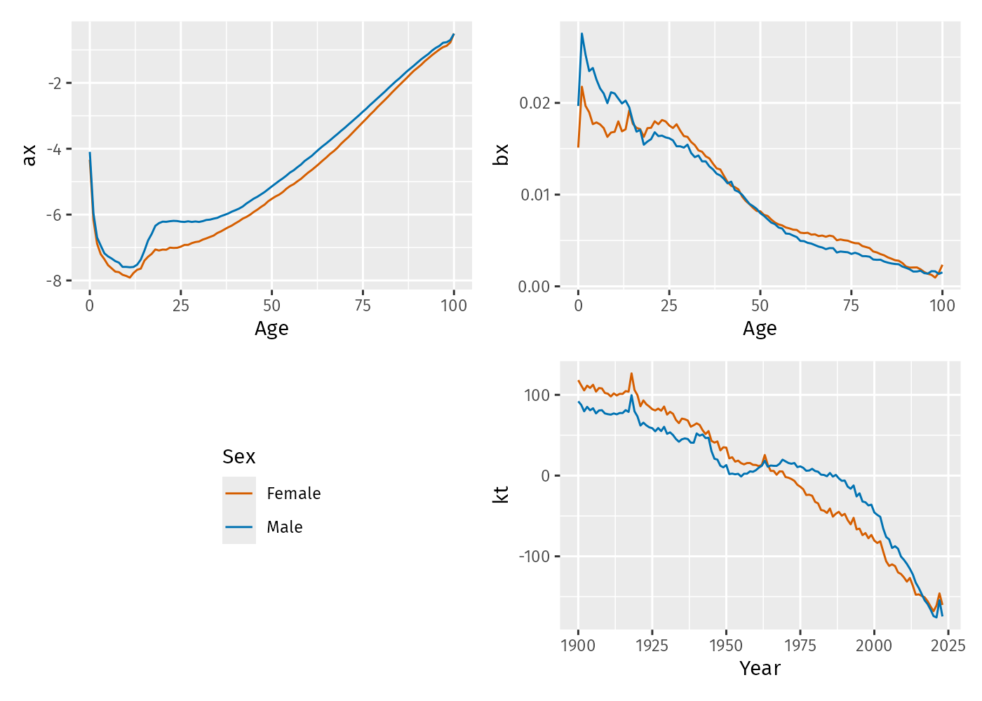
fit |>
  select(lee_carter) |>
  autoplot()

fit |>
  select(lee_carter) |>
  age_components()
#> # A tibble: 202 × 4
#>    Sex      Age    ax     bx
#>    <chr>  <int> <dbl>  <dbl>
#>  1 Female     0 -4.33 0.0151
#>  2 Female     1 -6.16 0.0218
#>  3 Female     2 -6.88 0.0197
#>  4 Female     3 -7.20 0.0190
#>  5 Female     4 -7.35 0.0177
#>  6 Female     5 -7.53 0.0179
#>  7 Female     6 -7.63 0.0177
#>  8 Female     7 -7.73 0.0173
#>  9 Female     8 -7.75 0.0163
#> 10 Female     9 -7.83 0.0168
#> # ℹ 192 more rows
fit |>
  select(lee_carter) |>
  time_components()
#> # A tsibble: 248 x 3 [1Y]
#> # Key:       Sex [2]
#>    Sex     Year    kt
#>    <chr>  <int> <dbl>
#>  1 Female  1900  118.
#>  2 Female  1901  112.
#>  3 Female  1902  105.
#>  4 Female  1903  111.
#>  5 Female  1904  109.
#>  6 Female  1905  113.
#>  7 Female  1906  104.
#>  8 Female  1907  108.
#>  9 Female  1908  108.
#> 10 Female  1909  102.
#> # ℹ 238 more rows

fit |> forecast(h = 20)
#> # A vital fable: 8,080 x 6 [1Y]
#> # Key:           Age x (Sex, .model) [101 x 4]
#>    Sex    .model      Year   Age          Mortality    .mean
#>    <chr>  <chr>      <int> <int>             <dist>    <dbl>
#>  1 Female lee_carter  2024     0 t(N(-6.8, 0.0087)) 0.00113
#>  2 Female lee_carter  2025     0  t(N(-6.8, 0.017)) 0.00110
#>  3 Female lee_carter  2026     0  t(N(-6.9, 0.026)) 0.00106
#>  4 Female lee_carter  2027     0  t(N(-6.9, 0.035)) 0.00103
#>  5 Female lee_carter  2028     0  t(N(-6.9, 0.045)) 0.00100
#>  6 Female lee_carter  2029     0    t(N(-7, 0.054)) 0.000973
#>  7 Female lee_carter  2030     0    t(N(-7, 0.064)) 0.000944
#>  8 Female lee_carter  2031     0    t(N(-7, 0.073)) 0.000917
#>  9 Female lee_carter  2032     0  t(N(-7.1, 0.083)) 0.000890
#> 10 Female lee_carter  2033     0  t(N(-7.1, 0.093)) 0.000864
#> # ℹ 8,070 more rows

The forecasts are returned as a distribution column (here transformed normal because of the log transformation used in the model). The .mean column gives the point forecasts equal to the mean of the distribution column.