Use XKCD's "Painbow" Colormap in ggplot2

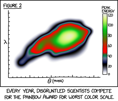
XKCD described a supposedly "bad" colormap that it called a "Painbow" (see < https://xkcd.com/2537/>). But simple tests demonstrate that under some circumstances, the colormap can perform very well, and people can find information that is difficult to detect with the ggplot2 default and even supposedly "good" colormaps like viridis. This library let's you use the Painbow in your own ggplot graphs.

Painbow

Painbow lets you use XKCD’s “painbow” colormap in ggplot.

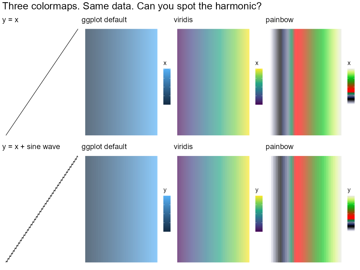
XKCD implied that this colormap is terrible, and even called it a “painbow”. However, these examples show that with certain tasks and data, this colormap outperforms even some of the most commonly cited “good” colormaps like viridis.

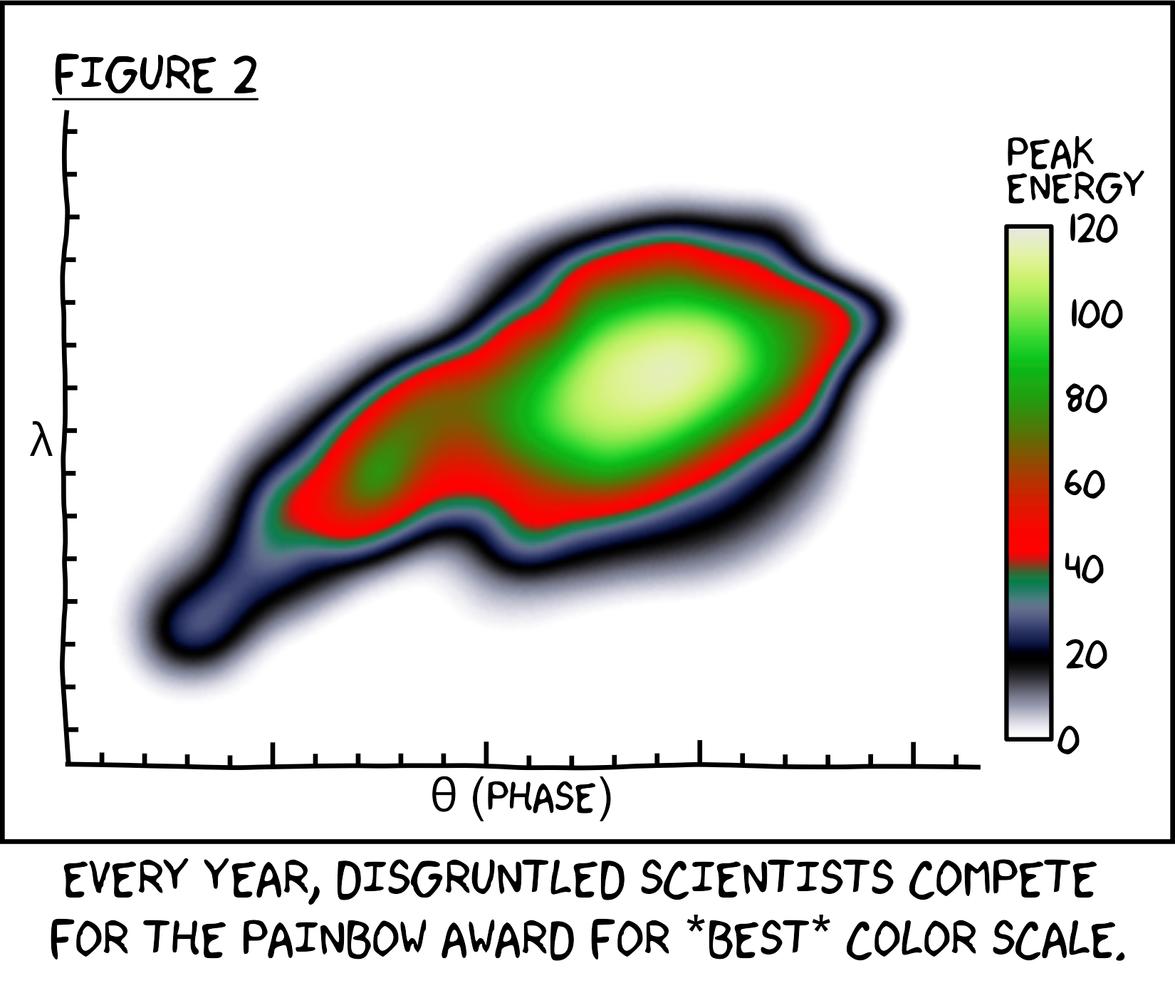
Here’s a reproduction in ggplot using some custom theming:

Installation

You can install the latest development version:

install.packages("devtools")
devtools::install_github("steveharoz/painbow")

Examples

Setup:

library(tidyverse)
library(painbow)
library(patchwork) # combine multiple graphs

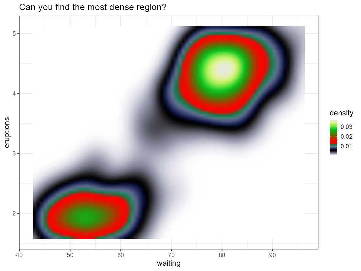
A simple example for the scale:

ggplot(faithfuld) +
  aes(waiting, eruptions, fill = density) +
  geom_raster(interpolate = TRUE) +
  scale_fill_painbow() +
  labs(title = "Can you find the most dense region?") +
  theme_bw(18)

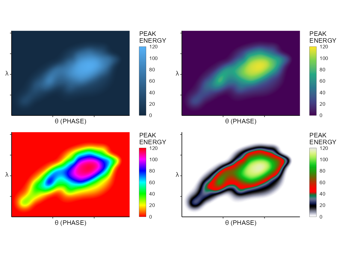
The dataset from the comic

The dataset is painbow_data. It was made using the comic’s image and a scripted lookup table.

Painbow may help you find outliers

Here is a 2D field with a regular pattern and a deviation. Can you find it? Painbow makes a task easier compared with commonly touted “good” colormaps.

##### 2D #####

COUNT = 512

data = expand.grid(
  x = 1:COUNT,
  y = 1:COUNT) %>% 
  mutate(z = sin(x/16) + cos(y/16)) %>% 
  mutate(znoise = z + dnorm(sqrt((x-0.75*COUNT)^2 + (y-0.33*COUNT)^2)/COUNT*20))

ggplot(data) +
  aes(x=x, y=y, fill=znoise) + 
  geom_raster() +
  labs(title = "ggplot default", fill=NULL) + 
  theme_void(15) + theme(legend.text = element_blank()) +
ggplot(data) +
  aes(x=x, y=y, fill=znoise) + 
  geom_raster() +
  scale_fill_viridis_c() +
  labs(title = "Viridis", fill=NULL) + 
  theme_void(15) + theme(legend.text = element_blank()) +
ggplot(data) +
  aes(x=x, y=y, fill=znoise) + 
  geom_raster() +
  scale_fill_painbow() +
  labs(title = "XKCD's colormap", fill=NULL) + 
  theme_void(15) + theme(legend.text = element_blank()) +
patchwork::plot_annotation(
  title = "Three colormaps. Same data. Can you spot the weird region?", 
  theme = theme(text = element_text(size=20)))

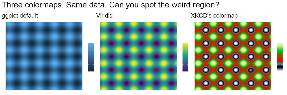
Painbow can help you spot a subtle pattern among data with high dynamic range

######## 1D #########

COUNT = 1024

data = tibble(
  x = 1:COUNT,
  y = x/COUNT + sin(x/4)/100
)

ggplot(data) +
  aes(x = x, y=x) + 
  geom_line() +
  labs(title = "y = x") + 
  theme_void(15) + theme(legend.text = element_blank()) +
ggplot(data) +
  aes(x = x, y=COUNT/2, fill=x) + 
  geom_tile(width=1, height=COUNT, color=NA) +
  labs(title = "ggplot default") + 
  theme_void(15) + theme(legend.text = element_blank()) +
ggplot(data) +
  aes(x = x, y=COUNT/2, fill=x) + 
  geom_tile(width=1, height=COUNT, color=NA) +
  scale_fill_viridis_c() +
  labs(title = "viridis") + 
  theme_void(15) + theme(legend.text = element_blank()) +
ggplot(data) +
  aes(x = x, y=COUNT/2, fill=x) + 
  geom_tile(width=1, height=COUNT, color=NA) +
  scale_fill_painbow() +
  labs(title = "painbow") + 
  theme_void(15) + theme(legend.text = element_blank()) +

ggplot(data) +
  aes(x = x, y=y) + 
  geom_line() +
  labs(title = "y = x + sine wave") +
  theme_void(15) + theme(legend.text = element_blank()) +
ggplot(data) +
  aes(x = x, y=COUNT/2, fill=y) + 
  geom_tile(width=1, height=COUNT, color=NA) +
  labs(title = "ggplot default") + 
  theme_void(15) + theme(legend.text = element_blank()) +
ggplot(data) +
  aes(x = x, y=COUNT/2, fill=y) + 
  geom_tile(width=1, height=COUNT, color=NA) +
  scale_fill_viridis_c() +
  labs(title = "viridis") + 
  theme_void(15) + theme(legend.text = element_blank()) +
ggplot(data) +
  aes(x = x, y=COUNT/2, fill=y) + 
  geom_tile(width=1, height=COUNT, color=NA) +
  scale_fill_painbow() +
  labs(title = "painbow") +
  theme_void(15) + theme(legend.text = element_blank()) +

patchwork::plot_layout(ncol=4) +
patchwork::plot_annotation(
    title = "Three colormaps. Same data. Can you spot the harmonic?", 
    theme = theme(text = element_text(size=20)))

Feedback, issues, and contributions

Feedback, suggestions, issues, and contributions are all welcome! Please file an issue or pull request at https://github.com/steveharoz/painbow/issues

Citing Painbow

The XKCD comic deserves credit: https://xkcd.com/2537/

Please cite this library via:
Steve Haroz (2021). Painbow. R package version 1.0.0, https://github.com/steveharoz/painbow/.