Efficient Bootstrap Methods for Block Maxima

Implements state-of-the-art block bootstrap methods for extreme value statistics based on block maxima. Includes disjoint blocks, sliding blocks, relying on a circular transformation of blocks. Fast C++ backends (via 'Rcpp') ensure scalability for large time series.

Welcome to maxbootR

The maxbootR package provides fast and consistent bootstrap methods for block maxima, designed for applications in extreme value statistics. Under the hood, performance-critical parts are implemented in C++ via Rcpp, enabling efficient computation even for long time series.

These methods are based on the first consistent bootstrap approach for block maxima as introduced in Bücher & Staud (2024+): Bootstrapping Estimators based on the Block Maxima Method..

Installation

You can install the development version of maxbootR from GitHub with:

# install.packages("devtools")
devtools::install_github("torbenstaud/maxbootR")

or from the official CRAN repository in R with:

install.packages("maxbootR")

Quick Example

The following example demonstrates how to extract sliding block maxima from synthetic data.

library(ggplot2)
library(maxbootR)
library(dplyr)

# Generate 100 years of daily observations
set.seed(91)
x <- rnorm(100 * 365)

# Extract sliding block maxima with 1-year window
bms <- blockmax(xx = x, block_size = 365, type = "sb")

# Create time-indexed tibble for plotting
df <- tibble(
  day = seq.Date(from = as.Date("1900-01-01"), by = "1 day", length.out = length(bms)),
  block_max = bms
)

# Plot the block maxima time series
ggplot(df, aes(x = day, y = block_max)) +
  geom_line(color = "steelblue") +
  labs(
    title = "Sliding Block Maxima from Simulated Data",
    x = "Year",
    y = "Block Maximum"
  ) 

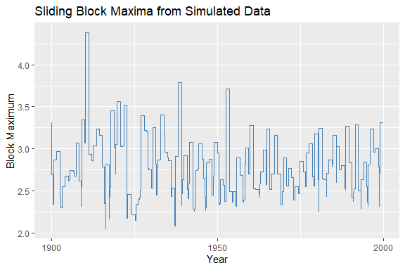
Time series of block maxima from simulated normal data

Bootstrap a 100-Year Return Level

We now use the maxbootr() function to bootstrap the 100-year return level of synthetic data, comparing the disjoint vs. sliding block bootstrap methods.

# Set block size (e.g., summer days)
bsize <- 92

# Generate synthetic time series
set.seed(1)
y <- rnorm(100 * bsize)

# Bootstrap using disjoint blocks (+timing)
system.time(
  bst.db <- maxbootr(xx = y, est = "rl", block_size = bsize, B = 500, 
                     type ="db", annuity = 100)
)
#>        User      System verstrichen 
#>        0.61        0.00        0.69

# Bootstrap using sliding blocks (+timing)
system.time(
  bst.sb <- maxbootr(xx = y, est = "rl", block_size = bsize, B = 500, 
                     type = "sb", annuity = 100)
)
#>        User      System verstrichen 
#>        6.86        0.00        6.89

# Compare variance
var(bst.sb) / var(bst.db)
#>           [,1]
#> [1,] 0.5502442

The sliding block method typically results in narrower bootstrap distributions, reducing statistical uncertainty.

Visualizing the Bootstrap Distribution

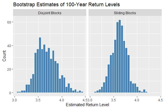
Histogram of return level bootstrap replicates

Learn More

For a full tutorial with real-world case studies (finance & climate), check out the vignette included in the package.

References

The implemented disjoint and sliding block bootstrap methods are grounded in the following foundational works:

• Gumbel, E. J. (1958). Statistics of Extremes. Columbia University Press.
• Ferro, C. A. T. & Segers, J. (2003). Inference for clusters of extreme values. Journal of the Royal Statistical Society: Series B (Statistical Methodology), 65(2), 545–556.

The block bootstrap methodology itself is based on:

• Bücher, A. & Staud, T. (2024+). Bootstrapping estimators based on the block maxima method. arXiv:2409.05529.

Roadmap & Future Development

I plan to further enhance maxbootR by:

• Adding functionality for computing (size-corrected) confidence intervals
• Providing built-in plotting and diagnostic functions
• Extending estimator support for multivariate block maxima

Your ideas and contributions are welcome — feel free to open an issue or pull request on GitHub!