Estimate Inverse Probability Weights

Functions to estimate the probability to receive the observed treatment, based on individual characteristics. The inverse of these probabilities can be used as weights when estimating causal effects from observational data via marginal structural models. Both point treatment situations and longitudinal studies can be analysed. The same functions can be used to correct for informative censoring.

ipw: Estimate Inverse Probability Weights

ipw

The ipw package provides a flexible toolkit for estimating Inverse Probability Weights (IPW) to fit marginal structural models. Functions to estimate the probability to receive the observed treatment, based on individual characteristics. The inverse of these probabilities can be used as weights when estimating causal effects from observational data via marginal structural models. Both point treatment situations and longitudinal studies can be analysed. The same functions can be used to correct for informative censoring.

Key Features

Point Treatment & Longitudinal Data: Functions to handle both static exposures and time-varying confounding.
Wide Range of Models: Support for binomial, multinomial, ordinal, and continuous (Gaussian) exposures.
Survival Analysis: Integration with Cox proportional hazards models for time-to-event data.
Diagnostic Tools: Built-in plotting functions to assess weight stability and the positivity assumption.

Installation

install.packages("ipw")

Example: Point Treatment Causal Inference

This example simulates data with a continuous confounder (l) and a binomial exposure (a) to estimate a marginal causal effect of 10.

library(ipw)
library(survey)

# 1. Simulate data
set.seed(123)
n <- 1000
simdat <- data.frame(l = rnorm(n, 10, 5))
a.lin <- simdat$l - 10
pa <- exp(a.lin)/(1 + exp(a.lin))
simdat$a <- rbinom(n, 1, prob = pa)
simdat$y <- 10*simdat$a + 0.5*simdat$l + rnorm(n, -10, 5)

# 2. Estimate IPW weights
temp <- ipwpoint(
   exposure = a,
   family = "binomial",
   link = "logit",
   numerator = ~ 1,
   denominator = ~ l,
   data = simdat)

# 3. Fit Marginal Structural Model (MSM)
msm <- svyglm(y ~ a, 
              design = svydesign(~1, weights = ~temp$ipw.weights, data = simdat))

summary(msm)
#> 
#> Call:
#> svyglm(formula = y ~ a, design = svydesign(~1, weights = ~temp$ipw.weights, 
#>     data = simdat))
#> 
#> Survey design:
#> svydesign(~1, weights = ~temp$ipw.weights, data = simdat)
#> 
#> Coefficients:
#>             Estimate Std. Error t value Pr(>|t|)    
#> (Intercept)  -6.2885     0.2757  -22.81   <2e-16 ***
#> a            10.6622     0.8083   13.19   <2e-16 ***
#> ---
#> Signif. codes:  0 '***' 0.001 '**' 0.01 '*' 0.05 '.' 0.1 ' ' 1
#> 
#> (Dispersion parameter for gaussian family taken to be 22.76977)
#> 
#> Number of Fisher Scoring iterations: 2

Example: Time-Varying Weights

For longitudinal research, such as analyzing TBM data, ipwtm calculates the cumulative product of weights over time.

library(ipw)
library(survival)

data(haartdat)

# Estimate time-varying weights for HAART initiation
temp_tm <- ipwtm(
  exposure = haartind,
  family = "survival",
  numerator = ~ sex + age,
  denominator = ~ sex + age + cd4.sqrt,
  id = patient,
  tstart = tstart,
  timevar = fuptime,
  type = "first",
  data = haartdat
)

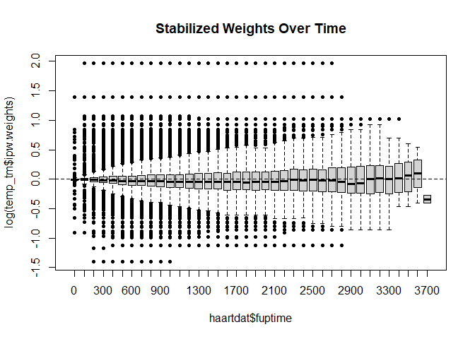
# Visualize weight stability
ipwplot(weights = temp_tm$ipw.weights, timevar = haartdat$fuptime, 
        binwidth = 100, main = "Stabilized Weights Over Time")

Authors

Hung Thai Tran - Research Assistant, Biostatistics Group at OUCRU.
Willem M. van der Wal - Original Author.
Ronald B. Geskus - Head of Biostatistics, OUCRU.

References

Van der Wal W.M. & Geskus R.B. (2011). ipw: An R Package for Inverse Probability Weighting. Journal of Statistical Software, 43(13), 1-23.
Robins J.M., Hernán M.A. & Brumback B.A. (2000). Marginal structural models and causal inference in epidemiology. Epidemiology, 11, 550-560.