Generalized Hypergeometric Function with Tunable High Precision

Computation of generalized hypergeometric function with tunable high precision in a vectorized manner, with the floating-point datatypes from 'mpfr' or 'gmp' library. The computation is limited to real numbers.

Generalized hypergeometric function with tunable high precision

Package: hypergeo2 0.2.0
Author: Xiurui Zhu
Modified: 2024-09-17 23:33:00
Compiled: 2024-10-14 22:55:54

The goal of hypergeo2 is to implement generalized hypergeometric function with tunable high precision. Two floating-point datatypes – mpfr_float and gmp_float – are channeled into this package. The computation is limited to real numbers, since its underlying workhorse boost::math::detail::hypergeometric_pFq_checked_series() from BH package implements comparisons (> or <) between numbers, which are not defined for complex datatypes.

Installation

System requirements

If you are building from source (e.g. not installing binaries on Windows), you need to prepare for two system requirements: ‘gmp’ and ‘mpfr’, to facilitate high-precision floating point types. You may follow the installation instructions from their websites, or try the following commands for quick (default) installation.

• For Windows with rtools40 (or newer) installed, please run:

pacman -Syu make pkg-config libtool gmp mpfr

• For macOS, please run:

brew install gmp mpfr

• For linux, please build and install platform-specific libraries through their configure file, or install them using conda.

If you are running R from an isolated environment (e.g. conda), you need to first activate the environment, and then build the system requirements and the package in the same environment to avoid version conflicts such as: undefined reference to memcpy@GLIBC#.#.#.

The package

If the requirements are installed into their default paths (e.g. without using the --prefix option), you are OK to go ahead installing the package in R, as pkg-config will take care finding them.

You can install the released version of hypergeo2 from CRAN with:

install.packages("hypergeo2")

Alternatively, you can install the developmental version of hypergeo2 from github with:

remotes::install_github("zhuxr11/hypergeo2")

However, if the requirements are not installed into their default paths, you may first need to provide configuration arguments/variables to installation paths. Optionally, you may also designate the maximal series iteration, default at 10000. To sum up, you may configure the installation in one of the following ways (replacing <my_gmp_install>, <my_mpfr_install> and <my_max_iter> with your paths) before installing the package with R CMD INSTALL in bash:

• Set --configure-args in R CMD INSTALL:

MY_GMP_INSTALL='<my_gmp_install>'
MY_MPFR_INSTALL='<my_mpfr_install>'
MY_MAX_ITER=<my_max_iter>
R CMD INSTALL hypergeo2 \
  --configure-args="\
    --with-gmp-include=${MY_GMP_INSTALL}/include \
    --with-mpfr-include=${MY_MPFR_INSTALL}/include \
    --with-gmp-lib=${MY_GMP_INSTALL}/lib \
    --with-mpfr-lib=${MY_MPFR_INSTALL}/lib \
    --with-max-iter=${MY_MAX_ITER}\
  "

• Set --configure-vars in R CMD INSTALL:

MY_GMP_INSTALL='<my_gmp_install>'
MY_MPFR_INSTALL='<my_mpfr_install>'
MY_MAX_ITER=<my_max_iter>
R CMD INSTALL hypergeo2 \
  --configure-vars="\
    GMP_INCLUDE=${MY_GMP_INSTALL}/include \
    MPFR_INCLUDE=${MY_MPFR_INSTALL}/include \
    GMP_LIB=${MY_GMP_INSTALL}/lib \
    MPFR_LIB=${MY_MPFR_INSTALL}/lib \
    MAX_ITER=${MY_MAX_ITER}\
  "

Examples of generalized hypergeometric function with tunable high precision

Sometimes, computing generalized hypergeometric function in double precision is not sufficient, even though we only need 6-8 accurate digits in the results. Here, two floating-point datatypes are provided: mpfr_float (“mpfr”) and gmp_float (“gmp”). By comparison, the “mpfr” backend is safer, since it defines while the “gmp” backend throws overflow exception. Therefore, mpfr_float is used as the default backend.

library(hypergeo2)

For example, let us compute a generalized hypergeometric function in Matlab Online and use its value as reference:

>> fprintf("%.32g", hypergeom([-28.2 11.8 15.8], [12.8 17.8], 1))
2.7120446907792120783054486094854e-09

First, we compute the same function with hypergeo::genhypergeo() function.

hypergeo_U <- c(-28.2, 11.8, 15.8)
hypergeo_L <- c(12.8, 17.8)
hypergeo_z <- 1
(hypergeo_res <- hypergeo::genhypergeo(U = hypergeo_U, L = hypergeo_L, z = hypergeo_z))
#> [1] 3.419707e-09

As can be seen, the result is heavily deviated by 0.261 in terms of relative error.

Then, we compute the same function with hypergeo2::genhypergeo() function, at default (double) precision.

(hypergeo2_res_double <- genhypergeo(U = hypergeo_U, L = hypergeo_L, z = hypergeo_z))
#> [1] 2.781375e-09

As can be seen, the result is still deviated by 0.0256 in terms of relative error, although much better.

Next, we compute the same function with hypergeo2::genhypergeo() function, with a precision of 20 digits from mpfr and gmp backends, respectively.

(hypergeo2_res_prec20_mpfr <- genhypergeo(U = hypergeo_U, L = hypergeo_L, z = hypergeo_z,
                                          prec = 20L, backend = "mpfr"))
#> [1] 2.712035e-09
(hypergeo2_res_prec20_gmp <- genhypergeo(U = hypergeo_U, L = hypergeo_L, z = hypergeo_z,
                                         prec = 20L, backend = "gmp"))
#> [1] 2.712045e-09

As can be seen, the result from gmp backend is more precise than that from mpfr, with the deviation of mpfr at -3.75e-06 and that of gmp at 2.68e-09. This is because that gmp usually use higher precision than we set (see this post).

Finally, to validate this hypothesis, we further increase the precision to 25 digits.

(hypergeo2_res_prec25_mpfr <- genhypergeo(U = hypergeo_U, L = hypergeo_L, z = hypergeo_z,
                                          prec = 25L, backend = "mpfr"))
#> [1] 2.712045e-09
(hypergeo2_res_prec25_gmp <- genhypergeo(U = hypergeo_U, L = hypergeo_L, z = hypergeo_z,
                                         prec = 25L, backend = "gmp"))
#> [1] 2.712045e-09

As can be seen, now both results are very close to the reference, with deviations from mpfr and gmp backends at 2.72e-09 and 2.68e-09, respectively.

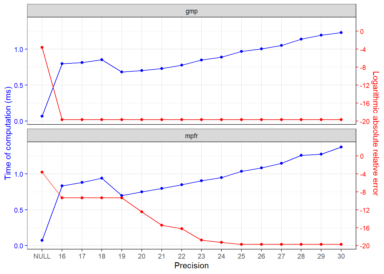
Precision vs time of computation

The time of computation at different precision is profiled in this section.

bench_scheme <- expand.grid(prec = c(list(NULL), as.list(seq(16L, 30L))),
                            backend = c("mpfr", "gmp"),
                            stringsAsFactors = FALSE)
bench_fun <- function(prec, backend, quote = FALSE) {
  res <- bquote(genhypergeo(U = hypergeo_U, L = hypergeo_L, z = hypergeo_z,
                            prec = .(prec), backend = .(backend)) / ref_value - 1)
  if (quote == FALSE) {
    eval(res)
  } else {
    res
  }
}
bench_scheme[["err"]] <- mapply(
  FUN = bench_fun,
  prec = bench_scheme[["prec"]],
  backend = bench_scheme[["backend"]],
  USE.NAMES = FALSE,
  SIMPLIFY = TRUE
)
bench_res <- summary(microbenchmark::microbenchmark(
  list = mapply(
    FUN = bench_fun,
    prec = bench_scheme[["prec"]],
    backend = bench_scheme[["backend"]],
    MoreArgs = list(quote = TRUE),
    USE.NAMES = FALSE,
    SIMPLIFY = TRUE
  ),
  times = 100L
))
bench_res <- cbind(bench_scheme, bench_res[colnames(bench_res) %in% "expr" == FALSE])
bench_res[["prec"]] <- as.character(bench_res[["prec"]])
ggplot2::ggplot(
  bench_res,
  ggplot2::aes(x = as.integer(factor(prec, levels = unique(prec))))
) +
  ggplot2::geom_point(ggplot2::aes(y = mean / 1000), color = "blue") +
  ggplot2::geom_line(ggplot2::aes(y = mean / 1000), color = "blue") +
  ggplot2::geom_point(ggplot2::aes(y = (log(abs(err)) + 20) / 16), color = "red") +
  ggplot2::geom_line(ggplot2::aes(y = (log(abs(err)) + 20) / 16), color = "red") +
  ggplot2::scale_x_continuous(breaks = seq_along(unique(bench_res[["prec"]])),
                              minor_breaks = NULL,
                              labels = unique(bench_res[["prec"]])) +
  ggplot2::scale_y_continuous(
    sec.axis = ggplot2::sec_axis(~. * 16 - 20,
                                 breaks = seq(-20, 0, by = 4),
                                 name = "Logarithmic absolute relative error")
  ) +
  ggplot2::facet_wrap(ggplot2::vars(backend), ncol = 1L) +
  ggplot2::theme_bw() +
  ggplot2::theme(
    axis.title.y.left = ggplot2::element_text(color = "blue"),
    axis.text.y.left = ggplot2::element_text(color = "blue"),
    axis.ticks.y.left = ggplot2::element_line(color = "blue"),
    axis.title.y.right = ggplot2::element_text(color = "red"),
    axis.text.y.right = ggplot2::element_text(color = "red"),
    axis.ticks.y.right = ggplot2::element_line(color = "red")
  ) +
  ggplot2::labs(x = "Precision", y = "Time of computation (ms)")