Add Vector Field Layers to Ggplots

Add vector field layers to ggplots. Ideal for visualising wind speeds, water currents, electric/magnetic fields, etc. Accepts data.frames, simple features (sf), and spatiotemporal arrays (stars) objects as input. Vector fields are depicted as arrows starting at specified locations, and with specified angles and radii.

ggfields

Overview

Add vector field layers to your ggplot2::ggplot(). Although it has similarities with ggplot2::geom_spoke(), ggfields offers some distinct features:

• The radius aesthetic is mapped to a scale and therefore can be added to the guides (see vignette("radius_aes")).
• Not only data.frames are supported, but also geometric data (sf::st_sf() and stars::st_as_stars()).
• Corrects angles for displayed aspect ratio or coordinate system (see vignette("angle_correction")).

Installation

Get CRAN version

install.packages("ggfields")

Get development version from r-universe

install.packages("ggfields", repos = c("https://pepijn-devries.r-universe.dev", "https://cloud.r-project.org"))

Adding vector fields to a map

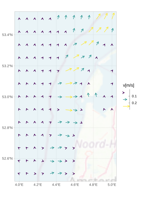
The example below shows how seawater current data can be added to a map:

library(ggplot2)
library(ggfields)
library(ggspatial) ## For annotating with Open Street Map

data(seawatervelocity)

ggplot() +
  ggspatial::annotation_map_tile(
    alpha      = 0.25,
    cachedir   = tempdir()) +
  geom_fields(
    data       = seawatervelocity,
    aes(radius = as.numeric(v),
        angle  = as.numeric(angle),
        colour = as.numeric(v)),
    max_radius = grid::unit(0.7, "cm")) +
  labs(colour  = "v[m/s]",
       radius  = "v[m/s]") +
  scale_radius_binned() +
  scale_colour_viridis_b(guide = guide_bins())

Simple data.frames

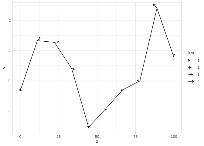
Vector arrows can also be added to simple plots with x and y data:

## First generate some arbitrary data to plot:
n  <- 10
df <- data.frame(x = seq(0, 100, length.out = n), y = rnorm(n),
                 ang = seq(0, 2*pi, length.out = n))
df$len <- 2 + df$y + rnorm(n)/4

ggplot(df, aes(x = x, y = y)) +
  geom_line() +
  geom_fields(aes(angle = ang, radius = len), .angle_correction = NULL)