forrest
Publication-Ready Forest Plots
Creates publication-ready forest plots from any tabular data containing point estimates and confidence intervals. Suitable for visualising results from regression models, meta-analyses, subgroup analyses, or any comparative study. Supports group and subgroup headings, summary estimates displayed as diamonds, grouped estimates with automatic colour and shape mapping, vertical dodging of multiple estimates within the same row, customisable text columns alongside the plot, and optional row striping. Provides a helper to export plots to PDF, PNG, SVG, or TIFF. Built on 'tinyplot' for clean, consistent visual styling with a minimal dependency footprint.
forrest 



forrest creates publication-ready forest plots from any data frame
that contains point estimates and confidence intervals — regression
models, subgroup analyses, meta-analyses, dose-response patterns, and
more. A single dependency
(tinyplot) keeps the
footprint minimal.
Key features:
- Works with any estimates and CIs: regression coefficients, ORs, HRs, MDs, …
- Automatic section headers from a grouping column (
sectionargument) — no manual NA rows - Two-level hierarchy with
subsectionfor nested grouping structures - Summary estimates rendered as filled diamonds (
is_summary) - Reference-category rows (NA estimate) rendered without CI, optionally
annotated with
" (Ref.)" - Alternating row stripes for readability (
stripe = TRUE) - Group colouring with automatic Okabe-Ito legend
- Optional text columns (formatted estimates, p-values, …) alongside the plot
- Section-level text column annotations via
section_cols - Log-scale x-axis for ratio measures
- CI clipping at axis limits with directional arrows
- Point size proportional to row weights
- Export to PDF, PNG, SVG, or TIFF with
save_forrest() - Works with
data.frame,tibble, anddata.table
Installation
install.packages("forrest")

# Development version from GitHub:
# install.packages("pak")
pak::pak("lorenzoFabbri/forrest")
Quick start
Introduction
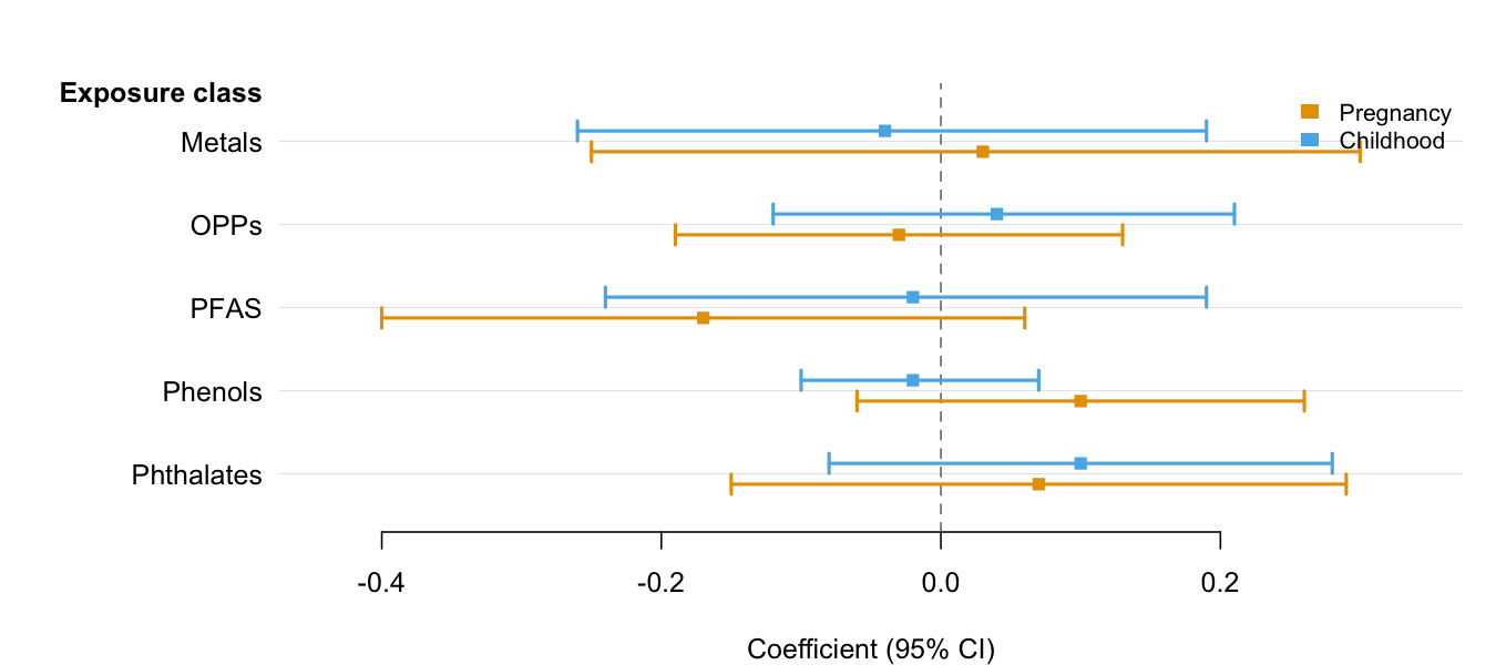
The minimal call requires only three column names — estimate, lower,
and upper. Use group and dodge = TRUE to place multiple CIs per
row when comparing results across categories (e.g., time periods, sexes,
models). See the Introduction
vignette
for the full feature tour.
library(forrest)

# Two estimates per exposure (e.g., two time windows)
periods <- data.frame(
  exposure = rep(c("Metals", "OPPs", "PFAS", "Phenols", "Phthalates"), each = 2),
  period   = rep(c("Pregnancy", "Childhood"), 5),
  est      = c( 0.03, -0.04, -0.03,  0.04, -0.17, -0.02,  0.10, -0.02,  0.07,  0.10),
  lo       = c(-0.25, -0.26, -0.19, -0.12, -0.40, -0.24, -0.06, -0.10, -0.15, -0.08),
  hi       = c( 0.30,  0.19,  0.13,  0.21,  0.06,  0.19,  0.26,  0.07,  0.29,  0.28)
)

forrest(
  periods,
  estimate = "est",
  lower    = "lo",
  upper    = "hi",
  label    = "exposure",
  group    = "period",
  dodge    = TRUE,
  header   = "Exposure class",
  ref_line = 0,
  xlab     = "Coefficient (95% CI)"
)
Meta-analysis
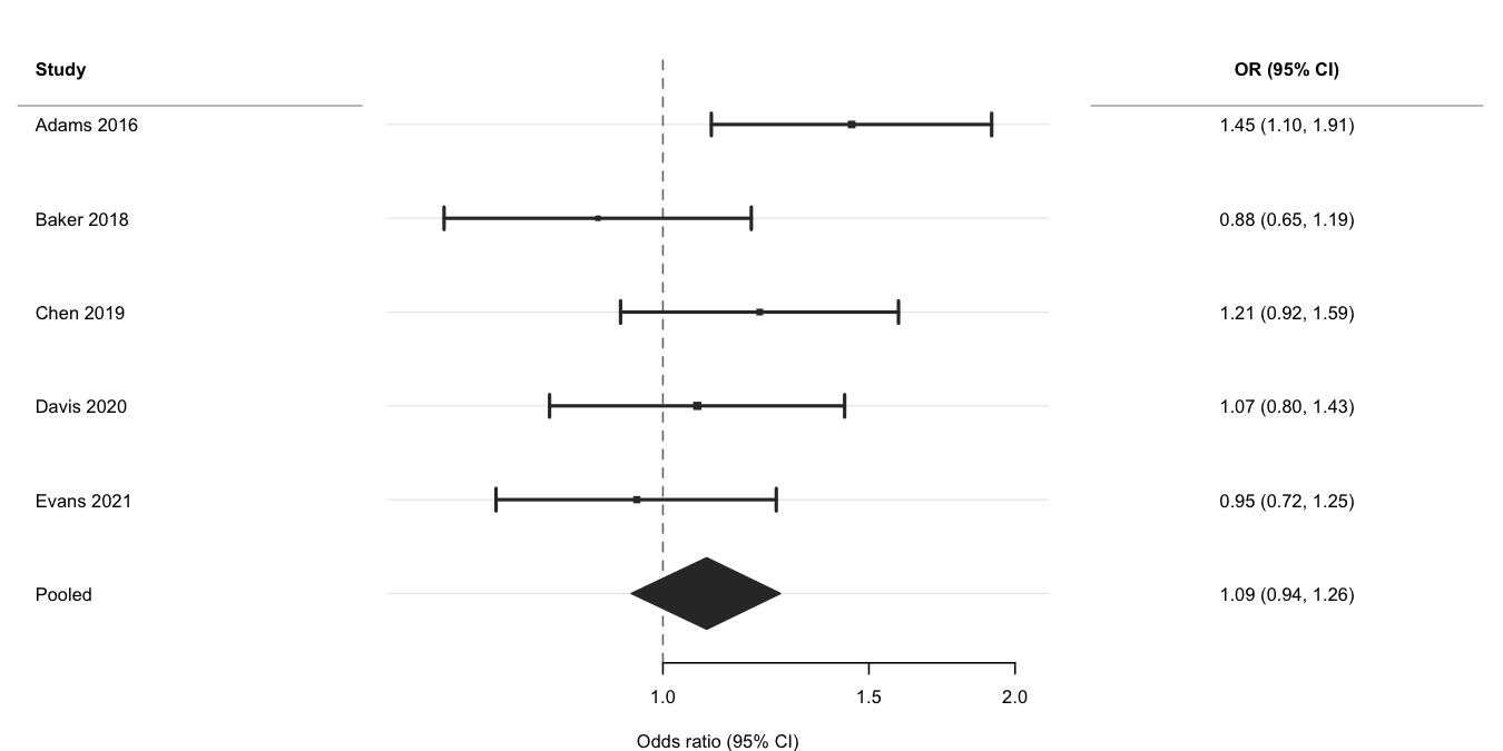
Use log_scale = TRUE and ref_line = 1 for ratio measures,
is_summary = TRUE to draw the pooled row as a filled diamond, and
weight to scale point sizes by inverse-variance weights. See the
Meta-analysis
vignette
for subgroup analyses and multi-exposure layouts.
ma <- data.frame(
  study  = c("Adams 2016", "Baker 2018", "Chen 2019",
             "Davis 2020", "Evans 2021", "Pooled"),
  est    = c(1.45, 0.88, 1.21, 1.07, 0.95, 1.09),
  lo     = c(1.10, 0.65, 0.92, 0.80, 0.72, 0.94),
  hi     = c(1.91, 1.19, 1.59, 1.43, 1.25, 1.26),
  weight = c(180, 95, 140, 210, 160, NA),
  is_sum = c(FALSE, FALSE, FALSE, FALSE, FALSE, TRUE)
)
ma$or_ci <- sprintf("%.2f (%.2f, %.2f)", ma$est, ma$lo, ma$hi)

forrest(
  ma,
  estimate   = "est",
  lower      = "lo",
  upper      = "hi",
  label      = "study",
  is_summary = "is_sum",
  weight     = "weight",
  log_scale  = TRUE,
  ref_line   = 1,
  header     = "Study",
  cols       = c("OR (95% CI)" = "or_ci"),
  widths     = c(2.2, 4, 2.5),
  xlab       = "Odds ratio (95% CI)"
)
Section headers
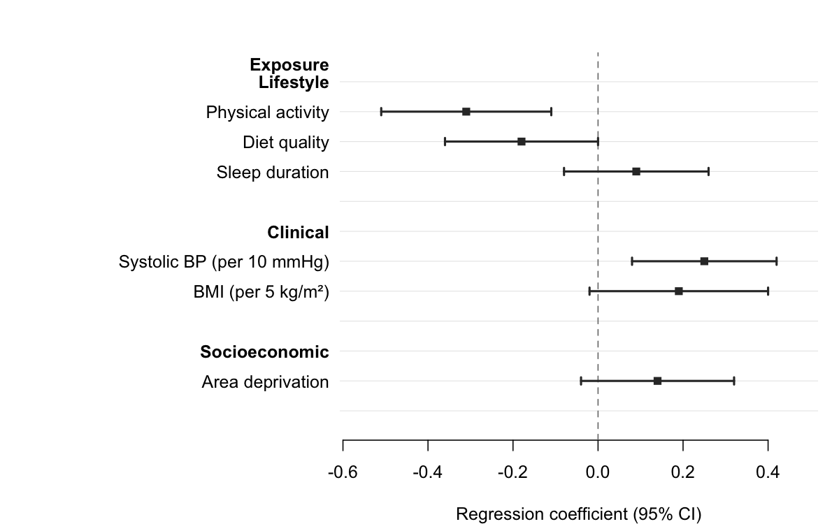
Pass a column name to section to group rows under automatic bold
headers. forrest() inserts a header wherever the section value
changes, indents the row labels, and adds a blank spacer after each
group — no manual data manipulation required.
subgroups <- data.frame(
  domain   = c("Lifestyle",  "Lifestyle",  "Lifestyle",
               "Clinical",   "Clinical",
               "Socioeconomic"),
  exposure = c("Physical activity", "Diet quality", "Sleep duration",
               "Systolic BP (per 10 mmHg)", "BMI (per 5 kg/m\u00b2)",
               "Area deprivation"),
  est      = c(-0.31, -0.18, 0.09, 0.25,  0.19, 0.14),
  lo       = c(-0.51, -0.36, -0.08, 0.08, -0.02, -0.04),
  hi       = c(-0.11, -0.00,  0.26, 0.42,  0.40,  0.32)
)

forrest(
  subgroups,
  estimate = "est",
  lower    = "lo",
  upper    = "hi",
  label    = "exposure",
  section  = "domain",
  header   = "Exposure",
  ref_line = 0,
  xlab     = "Regression coefficient (95% CI)"
)
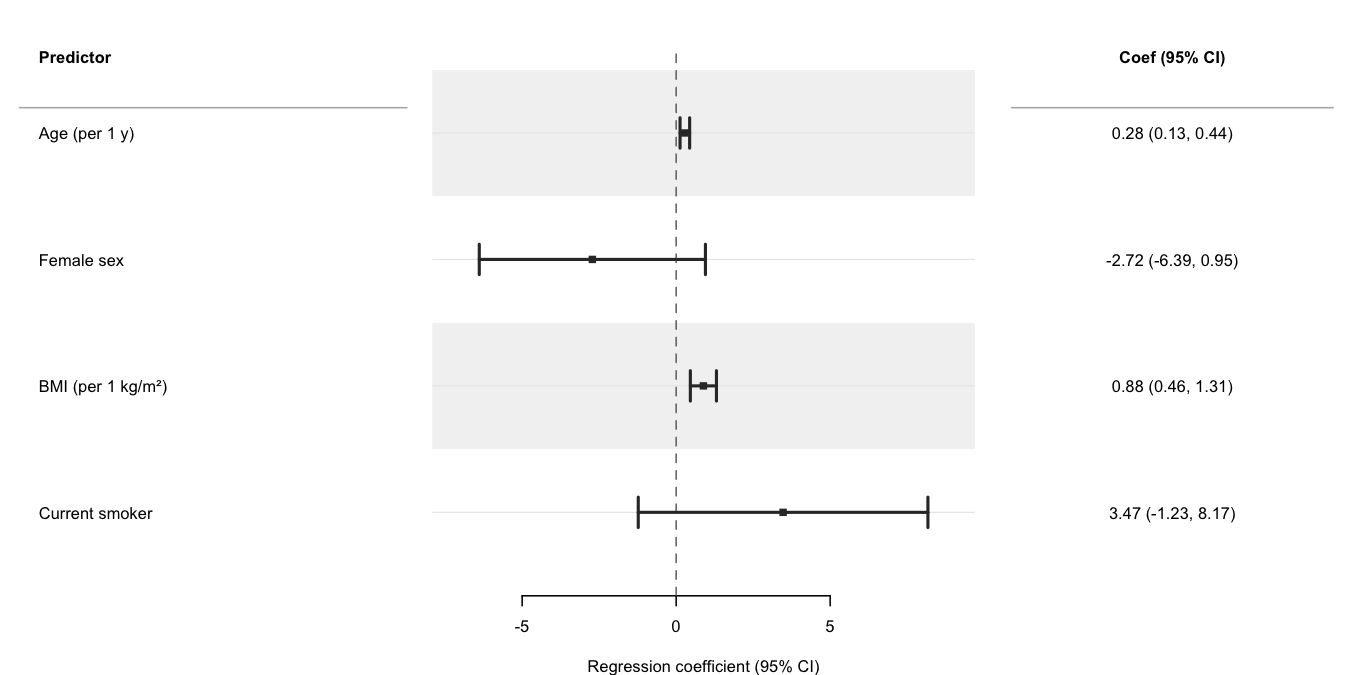
Regression models
Use broom::tidy() to extract
parameters from a fitted model and pass the result directly to
forrest(). The cols argument adds a formatted text column alongside
the plot; header labels the row-label panel. See the Regression
models
vignette
for progressive adjustment, multiple outcomes, dose-response, and causal
inference (g-computation, IPW) examples.
set.seed(1)
n   <- 300
dat <- data.frame(
  sbp    = 120 + rnorm(n, sd = 15),
  age    = runif(n, 30, 70),
  female = rbinom(n, 1, 0.5),
  bmi    = rnorm(n, 26, 4),
  smoker = rbinom(n, 1, 0.2)
)
dat$sbp <- dat$sbp + 0.3 * dat$age - 4 * dat$female +
           0.5 * dat$bmi - 2 * dat$smoker + rnorm(n, sd = 6)

fit   <- lm(sbp ~ age + female + bmi + smoker, data = dat)
coefs <- broom::tidy(fit, conf.int = TRUE)
coefs <- coefs[coefs$term != "(Intercept)", ]
coefs$term <- c("Age (per 1 y)", "Female sex",
                "BMI (per 1 kg/m²)", "Current smoker")

coefs$coef_ci <- sprintf(
  "%.2f (%.2f, %.2f)",
  coefs$estimate, coefs$conf.low, coefs$conf.high
)

forrest(
  coefs,
  estimate = "estimate",
  lower    = "conf.low",
  upper    = "conf.high",
  label    = "term",
  header   = "Predictor",
  cols     = c("Coef (95% CI)" = "coef_ci"),
  widths   = c(3, 4, 2.5),
  xlab     = "Regression coefficient (95% CI)",
  stripe   = TRUE
)
Compared with other packages
| Feature | forrest | forestplot | forestploter | ggforestplot |
|---|---|---|---|---|
| Minimal dependencies | ✅ | ❌ | ❌ | ❌ |
| General (not meta-analysis only) | ✅ | ✅ | ✅ | ⚠️ |
| Study weight sizing | ✅ | ✅ | ✅ | ❌ |
| Auto section headers from grouping column | ✅ | ⚠️ | ❌ | ❌ |
| Two-level nested section hierarchy | ✅ | ❌ | ❌ | ❌ |
| Summary diamonds | ✅ | ✅ | ✅ | ❌ |
| Text columns | ✅ | ✅ | ✅ | ❌ |
| Alternating row stripes | ✅ | ✅ | ✅ | ✅ |
| CI clipping with arrows | ✅ | ✅ | ⚠️ | ❌ |
| Group colouring + legend | ✅ | ✅ | ✅ | ✅ |
| Log-scale axis | ✅ | ✅ | ✅ | ✅ |
| Export helper | ✅ | ❌ | ⚠️ | ❌ |
| data.table support | ✅ | ❌ | ❌ | ❌ |
| Actively maintained | ✅ | ✅ | ✅ | ❌ |