Simulate Temporally Autocorrelated Populations

Temporally autocorrelated populations are correlated in their vital rates (growth, death, etc.) from year to year. It is very common for populations, whether they be bacteria, plants, or humans, to be temporally autocorrelated. This poses a challenge for stochastic population modeling, because a temporally correlated population will behave differently from an uncorrelated one. This package provides tools for simulating populations with white noise (no temporal autocorrelation), red noise (positive temporal autocorrelation), and blue noise (negative temporal autocorrelation). The algebraic formulation for autocorrelated noise comes from Ruokolainen et al. (2009) . Models for unstructured populations and for structured populations (matrix models) are available.

colorednoise

Overview

Many populations that change over time are temporally autocorrelated, which means that the random noise in each timestep is correlated to that of the previous timestep. Instead of uncorrelated white noise, these populations are governed by blue noise (negatively autocorrelated) or red noise (positively autocorrelated.)

The colorednoise package allows you to simulate colored noise as well as populations whose behavior is governed by colored noise.

Installation

You can install the latest version of colorednoise from github with:

# install.packages("devtools")
devtools::install_github("japilo/colorednoise")

Example

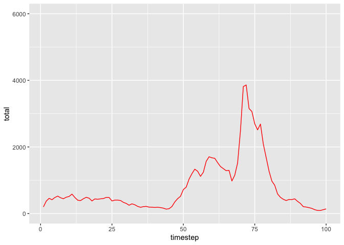
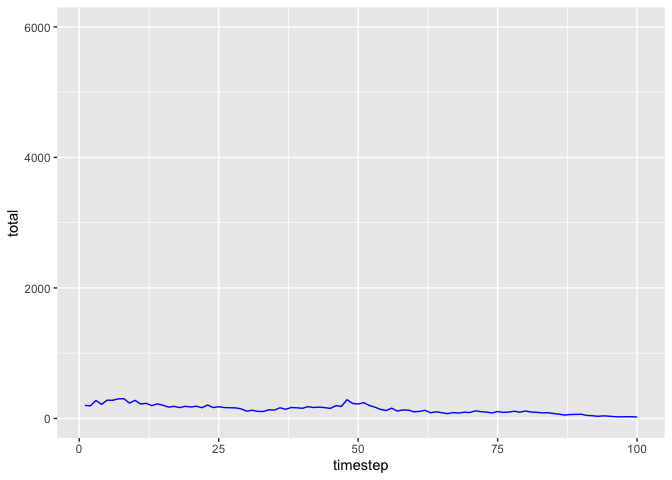
Here are plots of blue- and red-noise populations generated by the matrix_model function.

library(colorednoise)
set.seed(7927)
pop_blue <- matrix_model(
  data = list(
    mean = matrix(c(0.6687097, 0.2480645, 0.6687097, 0.4335484), ncol=2),
    sd = matrix(c(0.34437133, 0.08251947, 0.34437133, 0.10898160), ncol=2),
    autocorrelation = matrix(rep(-0.4, 4), ncol=2)
  ), timesteps = 100, initialPop = c(100, 100)
)
pop_red <- matrix_model(
  data = list(
    mean = matrix(c(0.6687097, 0.2480645, 0.6687097, 0.4335484), ncol=2),
    sd = matrix(c(0.34437133, 0.08251947, 0.34437133, 0.10898160), ncol=2),
    autocorrelation = matrix(rep(0.4, 4), ncol=2)
  ), timesteps = 100, initialPop = c(100, 100)
)
ggplot(pop_blue, aes(x = timestep, y = total)) + geom_line(col="blue") + ylim(0, 6000)

ggplot(pop_red, aes(x = timestep, y = total)) + geom_line(col="red") + ylim(0, 6000)