Calibration Bands

Package to assess the calibration of probabilistic classifiers using confidence bands for monotonic functions. Besides testing the classical goodness-of-fit null hypothesis of perfect calibration, the confidence bands calculated within that package facilitate inverted goodness-of-fit tests whose rejection allows for a sought-after conclusion of a sufficiently well-calibrated model. The package creates flexible graphical tools to perform these tests. For construction details see also Dimitriadis, Dümbgen, Henzi, Puke, Ziegel (2022) .

calibrationbands

An R package to assess calibration of binary outcome predictions. Authored by Timo Dimitriadis (Heidelberg University), Alexander Henzi (University of Bern), and Marius Puke (University of Hohenheim).

Installation

Development version

The most current version is available from GitHub.

# install.packages("devtools")
devtools::install_github("marius-cp/calibrationband")

Example

library(calibrationband)
library(dplyr)
set.seed(123)
s=.8
n=10000
x <- runif(n)
p <- function(x,s){p = 1/(1+((1/x*(1-x))^(s+1)));return(p)}
dat <- tibble::tibble(pr=x, s=s, cep = p(pr,s), y=rbinom(n,1,cep))%>% dplyr::arrange(pr)

cb <- calibration_bands(x=dat$pr, y=dat$y,alpha=0.05, method = "round", digits = 3)
print(cb) # prints autoplot and summary, see also autoplot(.) and summary(.)

#> Areas of misscalibration (ordered by length). In addition there are 1 more. 
#> # A tibble: 4 × 2
#>    min_x max_x
#>    <dbl> <dbl>
#> 1 0.0396 0.299
#> 2 0.693  0.951
#> 3 0.957  0.957
#> # … with 1 more row

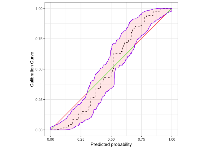
Use ggplot2:autolayer to customize the plot.

autoplot(cb,approx.equi=500, cut.bands = F,p_isoreg = NA,p_ribbon = NA,p_diag = NA)+
  ggplot2::autolayer(
    cb,
    cut.bands = F,
    p_diag = list(low = "green", high = "red", guide = "none", limits=c(0,1)),
    p_isoreg = list(linetype = "dashed"),
    p_ribbon = list(alpha = .1, fill = "red", colour = "purple")
                     )

```