Tools for Conservation Science

Provides data science tools for conservation science, including methods for environmental data analysis, humidity calculations, sustainability metrics, engineering calculations, and data visualisation. Supports conservators, scientists, and engineers working with cultural heritage preventive conservation data. The package is motivated by the framework outlined in Cosaert and Beltran et al. (2022) "Tools for the Analysis of Collection Environments" < https://www.getty.edu/conservation/publications_resources/pdf_publications/tools_for_the_analysis_of_collection_environments.html>.

ConSciR

ConSciR provides tools for the analysis of cultural heritage preventive conservation data.

It includes functions for environmental data analysis, humidity calculations, sustainability metrics, conservation risks, and data visualisations such as psychrometric charts. It is designed to support conservators, scientists, and engineers by streamlining common calculations and tasks encountered in heritage conservation workflows. The package is motivated by the framework outlined in Cosaert and Beltran et al. (2022) “Tools for the Analysis of Collection Environments” “Tools for the Analysis of Collection Environments”.

ConSciR is intended for:

• Conservators working in museums, galleries, and heritage sites
• Conservation scientists, engineers, and researchers
• Data scientists developing applications for conservation
• Cultural heritage professionals involved in preventive conservation
• Students and educators in conservation and heritage science programmes

The package is also designed to be:

• FAIR: Findable, Accessible, Interoperable, and Reusable
• Collaborative: enabling contributions, feature requests, bug reports, and additions from the wider community

If using R for the first time, read an article here: Using R for the first time

Tools

• Humidity calculations, conservator tools, and sustainability metrics.
• Mould growth models and damage risk functions.
• Graphical outputs including temperature-relative humidity (TRH) plots, psychrometric charts and data for other applications.
• Data tidying functions compatible with Meaco and Hanwell environmental monitoring devices.
• Interactive Shiny applications enabling dynamic data exploration and visualisation.

Install and load

install.packages("ConSciR")
library(ConSciR)

You can install the development version of the package from GitHub using the pak package:

install.packages("pak")
pak::pak("BhavShah01/ConSciR")

# Alternatively
# install.packages("devtools")
# devtools::install_github("BhavShah01/ConSciR")

For full details on all functions, see the package Reference manual.

Examples

This section demonstrates some common tasks you can perform with the ConSciR package.

• Load packages
  Load ConSciR and some commonly used tidyverse packages for data manipulation and plotting.

library(ConSciR)
library(dplyr)
library(ggplot2)

• Access an example dataset
  A pre-loaded dataset (mydata) is included for testing and demonstration. Use head() to view the first few rows and inspect the data structure.
• Users can rename columns and structure their own datasets similarly to mydata to ensure compatibility with ConSciR functions, which expect variables such as temperature and relative humidity in specific column names.

# My TRH data
filepath <- data_file_path("mydata.xlsx")
mydata <- readxl::read_excel(filepath, sheet = "mydata")
mydata <- mydata |> filter(Sensor == "Room 1")

head(mydata)
#> # A tibble: 6 × 5
#>   Site   Sensor Date                 Temp    RH
#>   <chr>  <chr>  <dttm>              <dbl> <dbl>
#> 1 London Room 1 2024-01-01 00:00:00  21.8  36.8
#> 2 London Room 1 2024-01-01 00:15:00  21.8  36.7
#> 3 London Room 1 2024-01-01 00:29:59  21.8  36.6
#> 4 London Room 1 2024-01-01 00:44:59  21.7  36.6
#> 5 London Room 1 2024-01-01 00:59:59  21.7  36.5
#> 6 London Room 1 2024-01-01 01:14:59  21.7  36.2

• Perform calculations on the data
  Use ConSciR functions to add metrics such as dew point, absolute humidity, mould, preservation index and others to the dataset. More functions are available; see the package Reference for details.

# Peform calculations
head(mydata) |>
  mutate(
    # Dew point
    DewP = calcDP(Temp, RH), 
    
    # Absolute humidity
    Abs = calcAH(Temp, RH), 
    
    # Mould risk 
    Mould = ifelse(RH > calcMould_Zeng(Temp, RH), "Mould risk", "No mould"), 
    
    # Preservation Index, years to deterioration 
    PI = calcPI(Temp, RH), 
    
    # Scenario: Humidity if the temperature was 2°C higher
    RH_if_2C_higher = calcRH_AH(Temp + 2, Abs) 
    ) |>
  glimpse()
#> Rows: 6
#> Columns: 10
#> $ Site            <chr> "London", "London", "London", "London", "London", "Lon…
#> $ Sensor          <chr> "Room 1", "Room 1", "Room 1", "Room 1", "Room 1", "Roo…
#> $ Date            <dttm> 2024-01-01 00:00:00, 2024-01-01 00:15:00, 2024-01-01 …
#> $ Temp            <dbl> 21.8, 21.8, 21.8, 21.7, 21.7, 21.7
#> $ RH              <dbl> 36.8, 36.7, 36.6, 36.6, 36.5, 36.2
#> $ DewP            <dbl> 6.383970, 6.344456, 6.304848, 6.216205, 6.176529, 6.05…
#> $ Abs             <dbl> 7.052415, 7.033251, 7.014087, 6.973723, 6.954670, 6.89…
#> $ Mould           <chr> "No mould", "No mould", "No mould", "No mould", "No mo…
#> $ PI              <dbl> 45.25849, 45.38181, 45.50580, 46.07769, 46.20393, 46.5…
#> $ RH_if_2C_higher <dbl> 32.81971, 32.73052, 32.64134, 32.63838, 32.54920, 32.2…

• Combine analysis with visualisation
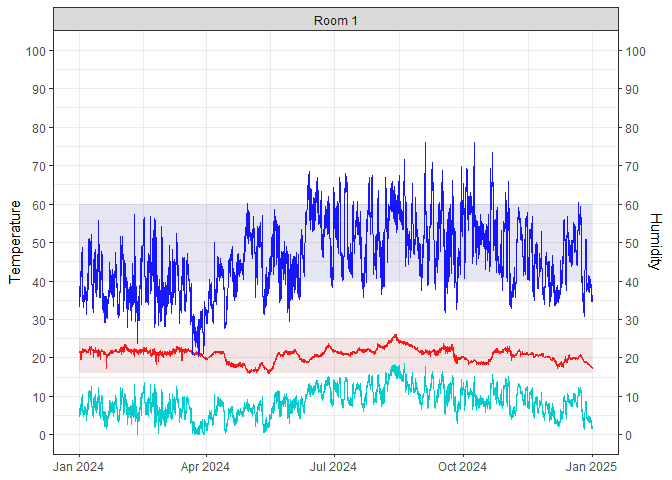
  Add a dew point line to the temperature-relative humidity graph using the package’s built-in plotting function graph_TRH().

mydata |>
  mutate(DewPoint = calcDP(Temp, RH)) |>
  graph_TRH() + 
  geom_line(aes(Date, DewPoint), col = "cyan3") + # add dew point 
  theme_bw()

• Conservator tools: mould growth estimation
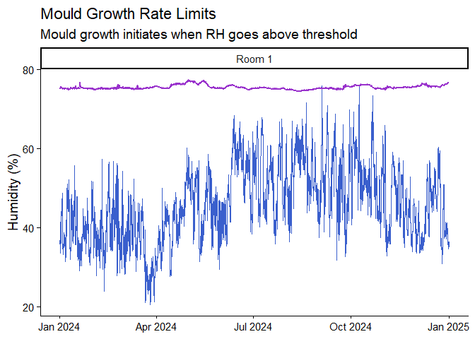
  Calculate mould growth risk using calcMould_Zeng() function and visualise it alongside humidity data.

mydata |>
  mutate(Mould = calcMould_Zeng(Temp, RH)) |>
  ggplot() +
  geom_line(aes(Date, RH), col = "royalblue3") +
  geom_line(aes(Date, Mould), col = "darkorchid", size = 1) +
  labs(title = "Mould Growth Rate Limits", 
       subtitle = "Mould growth initiates when RH goes above threshold",
       x = NULL, y = "Humidity (%)") +
  facet_grid(~Sensor) + 
  theme_classic(base_size = 14)

• Graphs: generate a psychrometric chart
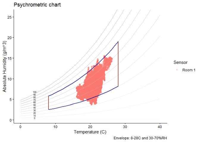
  Visualise the data using a psychrometric chart with the function graph_psychrometric(). The example shows how a basic plot can be customised; data transparency, temperature and humidity ranges, and the y-axis function.

# Customise 
mydata |>
  graph_psychrometric(
    data_alpha = 0.2,
    LowT = 8, 
    HighT = 28,
    LowRH = 30,
    HighRH = 70,
    y_func = calcAH
    ) +
  theme_classic() + 
  labs(title = "Psychrometric chart")