tablespan
Create Satisficing 'Excel', 'HTML', 'LaTeX', and 'RTF' Tables using a Simple Formula
Create "good enough" tables with a single formula. 'tablespan' tables can be exported to 'Excel', 'HTML', 'LaTeX', and 'RTF' by leveraging the packages 'openxlsx' and 'gt'. See < https://jhorzek.github.io/tablespan/> for an introduction.
tablespan

Create satisficing tables in R the formula way.
The objective of tablespan is to provide a “good enough” approach to
creating tables by leveraging R’s formulas.
The following shows an example, where we define a relatively complex table header setup with a single formula. The details of the syntax will be explained below.
library(dplyr)
library(tablespan)
data("mtcars")

summarized_table <- mtcars |>
  group_by(cyl, vs) |>
  summarise(N = n(),
            mean_hp = mean(hp),
            sd_hp = sd(hp),
            mean_wt = mean(wt),
            sd_wt = sd(wt))
#> `summarise()` has grouped output by 'cyl'. You can override using the `.groups`
#> argument.

tbl <- tablespan(data = summarized_table,
                 formula = Cylinder:cyl + Engine:vs ~
                   N +
                   (`Horse Power` = Mean:mean_hp + SD:sd_hp) +
                   (`Weight` = Mean:mean_wt + SD:sd_wt),
                 title = "Motor Trend Car Road Tests",
                 subtitle = "A table created with tablespan",
                 footnote = "Data from the infamous mtcars data set.")
tbl
#> Motor Trend Car Road Tests
#> A table created with tablespan
#>
#>  |                 |     Horse Power       Weight      |
#>  | Cylinder Engine | N   Mean        SD    Mean   SD   |
#>  | -------- ------ - --  ----------- ----- ------ ---- |
#>  | 4        0      | 1   91                2.14        |
#>  | 4        1      | 10  81.8        21.87 2.3    0.6  |
#>  | 6        0      | 3   131.67      37.53 2.76   0.13 |
#>  | ...      ...    | ... ...         ...   ...    ...  |
#> Data from the infamous mtcars data set.
tablespan builds on the awesome packages
openxlsx and
gt, which allows tables created with
tablespan to be exported to the following formats:
Installation
To install tablespan from CRAN use:
install.packages("tablespan")
The development version of tablespan can be installed from GitHub
with:
library(remotes)
remotes::install_github("jhorzek/tablespan")
Introduction
R has a large set of great packages that allow you to create and export
tables that look exactly like you envisioned. However, sometimes you may
just need a good-enough table that is easy to create and share with
others. This is where tablespan can be of help.
Let’s assume that we want to share the following table:
library(dplyr)
data("mtcars")

summarized_table <- mtcars |>
  group_by(cyl, vs) |>
  summarise(N = n(),
            mean_hp = mean(hp),
            sd_hp = sd(hp),
            mean_wt = mean(wt),
            sd_wt = sd(wt))
#> `summarise()` has grouped output by 'cyl'. You can override using the `.groups`
#> argument.

print(summarized_table)
#> # A tibble: 5 × 7
#> # Groups:   cyl [3]
#>     cyl    vs     N mean_hp sd_hp mean_wt  sd_wt
#>   <dbl> <dbl> <int>   <dbl> <dbl>   <dbl>  <dbl>
#> 1     4     0     1    91   NA       2.14 NA
#> 2     4     1    10    81.8 21.9     2.30  0.598
#> 3     6     0     3   132.  37.5     2.76  0.128
#> 4     6     1     4   115.   9.18    3.39  0.116
#> 5     8     0    14   209.  51.0     4.00  0.759
We don’t want to share the table as is - the variable names are all a bit technical and the table could need some spanners summarizing columns. So, we want to share a table that looks something like this:
|                   | Horse Power |   Weight  |
| Cylinder | Engine | Mean  |  SD | Mean | SD |
| -------- | ------ | ----- | --- | ---- | -- |
|                   |                         |
tablespan allows us to create this table with a single formula.
Creating a Basic Table
In tablespan, the table headers are defined with a formula. For
example, cyl ~ mean_hp + sd_hp defines a table with cyl as the row
names and mean_hp and sd_hp as columns:
library(tablespan)
tablespan(data = summarized_table,
          formula = cyl ~ mean_hp + sd_hp)
#>
#>  | cyl | mean_hp sd_hp |
#>  | --- - ------- ----- |
#>  | 4   | 91            |
#>  | 4   | 81.8    21.87 |
#>  | 6   | 131.67  37.53 |
#>  | ... | ...     ...   |
Note that the row names (cyl) are in a separate block to the left.
Adding Spanners
Spanners are defined using braces and spanner names. For example, the
following defines a spanner for mean_hp and sd_hp with the name
Horsepower: cyl ~ (Horsepower = mean_hp + sd_hp):
tablespan(data = summarized_table,
          formula = cyl ~ (Horsepower = mean_hp + sd_hp))
#>
#>  |     | Horsepower       |
#>  | cyl | mean_hp    sd_hp |
#>  | --- - ---------- ----- |
#>  | 4   | 91               |
#>  | 4   | 81.8       21.87 |
#>  | 6   | 131.67     37.53 |
#>  | ... | ...        ...   |
Spanners can also be nested:
tablespan(data = summarized_table,
          formula = cyl ~ (Horsepower = (Mean = mean_hp) + (SD  = sd_hp)))
#>
#>  |     | Horsepower       |
#>  |     | Mean       SD    |
#>  | cyl | mean_hp    sd_hp |
#>  | --- - ---------- ----- |
#>  | 4   | 91               |
#>  | 4   | 81.8       21.87 |
#>  | 6   | 131.67     37.53 |
#>  | ... | ...        ...   |
Renaming Columns
Variable names in an R data.frame are often very technical (e.g.,
mean_hp and sd_hp). When sharing the table, we may want to replace
those names. In the example above, we may want to replace mean_hp and
sd_hp with “Mean” and “SD”. In tablespan renaming variables is
achieved with new_name:old_name. For example,
cyl ~ (Horsepower = Mean:mean_hp + SD:sd_hp) renames mean_hp to
Mean and sd_hp to SD:
tablespan(data = summarized_table,
          formula = cyl ~ (Horsepower = Mean:mean_hp + SD:sd_hp))
#>
#>  |     | Horsepower       |
#>  | cyl | Mean       SD    |
#>  | --- - ---------- ----- |
#>  | 4   | 91               |
#>  | 4   | 81.8       21.87 |
#>  | 6   | 131.67     37.53 |
#>  | ... | ...        ...   |
Creating the Full Table
The combination of row names, spanners, and renaming of variables allows creating the full table:
library(dplyr)
library(tablespan)
data("mtcars")

summarized_table <- mtcars |>
  group_by(cyl, vs) |>
  summarise(N = n(),
            mean_hp = mean(hp),
            sd_hp = sd(hp),
            mean_wt = mean(wt),
            sd_wt = sd(wt))
#> `summarise()` has grouped output by 'cyl'. You can override using the `.groups`
#> argument.

tbl <- tablespan(data = summarized_table,
                 formula = Cylinder:cyl + Engine:vs ~
                   N +
                   (`Horse Power` = Mean:mean_hp + SD:sd_hp) +
                   (`Weight` = Mean:mean_wt + SD:sd_wt),
                 title = "Motor Trend Car Road Tests",
                 subtitle = "A table created with tablespan",
                 footnote = "Data from the infamous mtcars data set.")
tbl
#> Motor Trend Car Road Tests
#> A table created with tablespan
#>
#>  |                 |     Horse Power       Weight      |
#>  | Cylinder Engine | N   Mean        SD    Mean   SD   |
#>  | -------- ------ - --  ----------- ----- ------ ---- |
#>  | 4        0      | 1   91                2.14        |
#>  | 4        1      | 10  81.8        21.87 2.3    0.6  |
#>  | 6        0      | 3   131.67      37.53 2.76   0.13 |
#>  | ...      ...    | ... ...         ...   ...    ...  |
#> Data from the infamous mtcars data set.
Tables without row names
Using 1 on the left hand side of the formula creates a table without
row names. For example, 1 ~ (Horsepower = Mean:mean_hp + SD:sd_hp)
defines:
tablespan(data = summarized_table,
          formula = 1 ~ (Horsepower = Mean:mean_hp + SD:sd_hp))
#>
#>  | Horsepower       |
#>  | Mean       SD    |
#>  | ---------- ----- |
#>  | 91               |
#>  | 81.8       21.87 |
#>  | 131.67     37.53 |
#>  | ...        ...   |
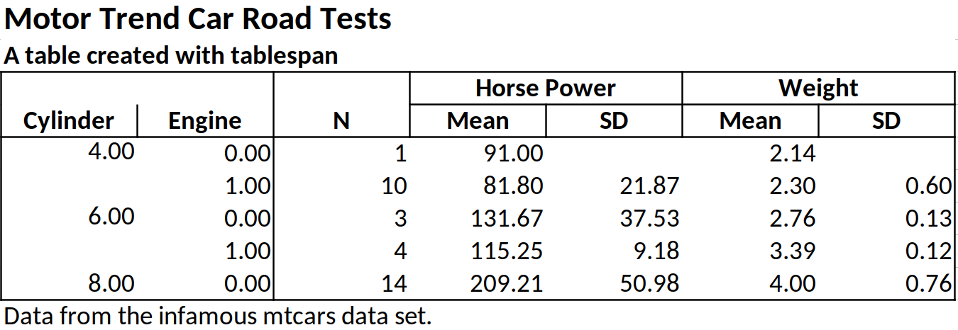
Exporting to Excel
Tables created with tablespan can now be translated to xlsx tables
with openxlsx using the
as_excel function:
# as_excel creates an openxlsx workbook
wb <- as_excel(tbl = tbl)

# Save the workbook as an xlsx file:
# openxlsx::saveWorkbook(wb,
#                        file = "cars.xlsx",
#                        overwrite = TRUE)
Exporting to HTML, LaTeX, and RTF
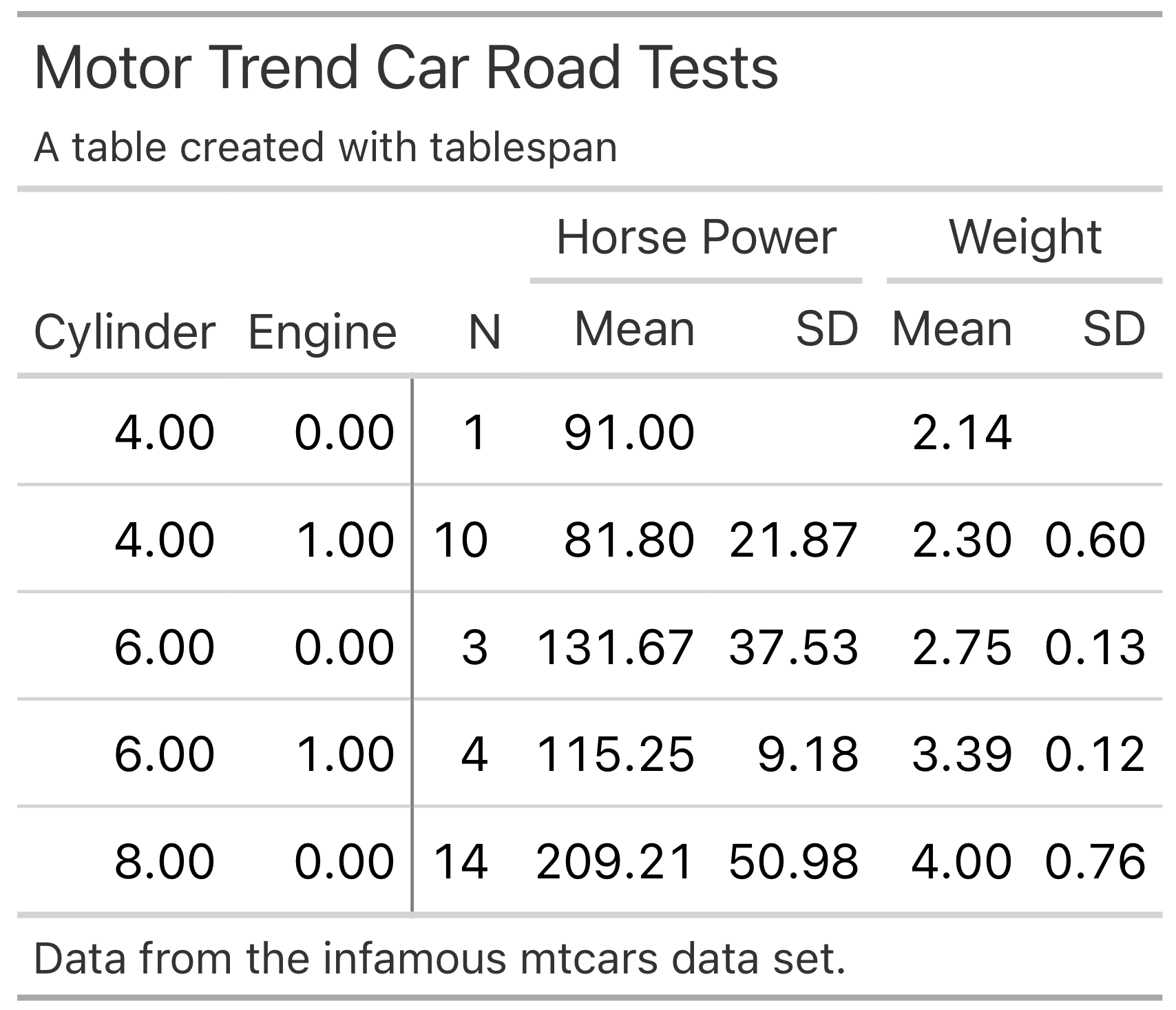
Tables created with tablespan can also be exported to gt which
allows saving as HTML, LaTeX, or RTF file. To this end, we simply have
to call as_gt on our table:
# Translate to gt:
gt_tbl <- as_gt(tbl = tbl)
gt_tbl
Styling
tablespan allows adding styles to tables that are automatically
exported to gt and openxlsx. The workflow is heavily inspired by
gt.
All functions used to style tablespan tables start with style_:
style_title: Adapt the style of the titlestyle_subtitle: Adapt the style of the subtitlestyle_header: Adapt the style of the headerstyle_header_cells: Stlye the header cells in openxlsx. Used to create the borders around header cells (only relevant for openxlsx exports)style_column: Add styling to the body of the tablestyle_footnote: Adapt the style of the footnotesstyle_vline: Adapt the style of the vertical lines in the table. Only relevant for openxlsxstyle_hline: Adapt the style of the horizontal lines in the table. Only relevant for openxlsx
Styling the title and subtitle
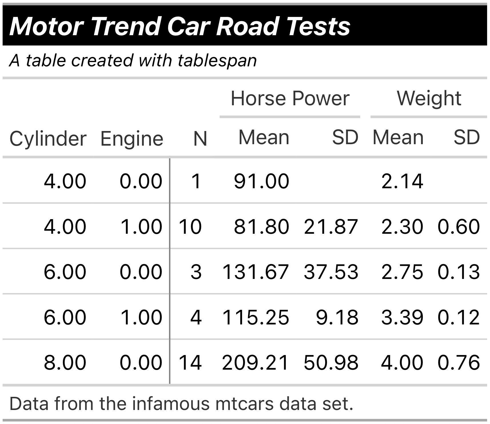
Use the style_title and style_subtitle options to style title and
subtitle:
tbl |>
  style_title(background_color = "#000000",
              text_color = "#ffffff",
              bold = TRUE,
              italic = TRUE) |>
  style_subtitle(italic = TRUE) |>
  as_gt()
All of the styles applied in the following would also be exported to
.xlsx files when using as_excel and saving the workbook with
openxlsx.
Styling the header
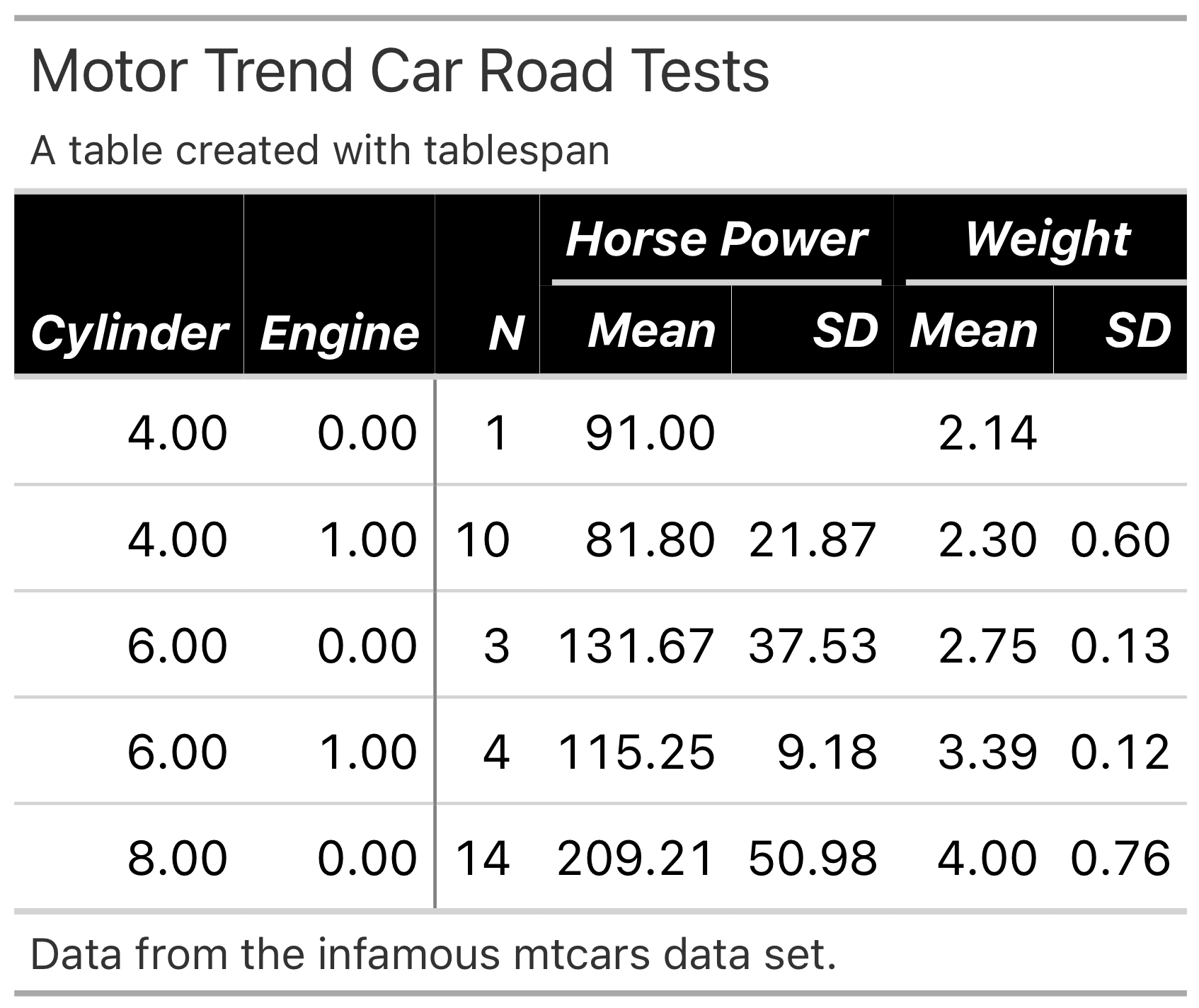
To adapt the header, use style_header:
tbl |>
  style_header(background_color = "#000000",
               text_color = "#ffffff",
               bold = TRUE,
               italic = TRUE) |>
  as_gt()
Styling the body
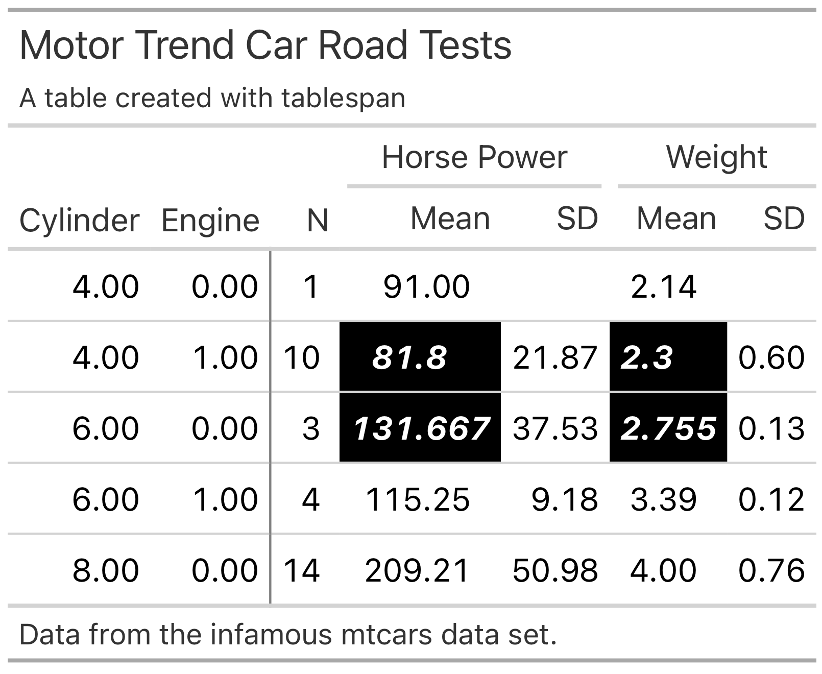
The body is adapted with style_column. This function also allows
styling only specific cells in the body or styling multiple columns at
once. Columns are selected with tidy expressions. Please note that you
will have to reference the columns with their respective names in the
raw data set, not the names shown in the spanner:
tbl |>
  style_column(
    columns = starts_with("mean_"),
    rows = 2:3,
    background_color = "#000000",
    text_color = "#ffffff",
    bold = TRUE,
    italic = TRUE) |>
  as_gt()
Styling the footnote
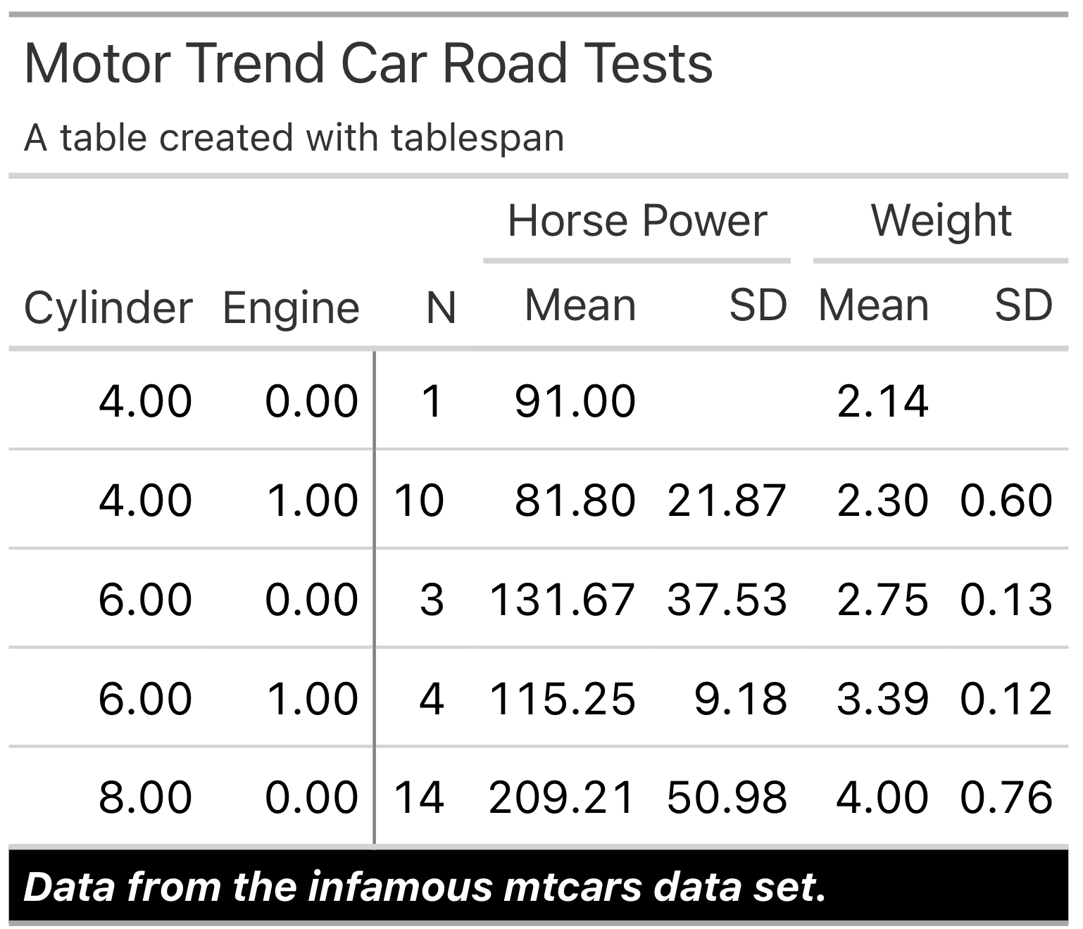
tbl |>
  style_footnote(
    background_color = "#000000",
    text_color = "#ffffff",
    bold = TRUE,
    italic = TRUE) |>
  as_gt()
Custom styles
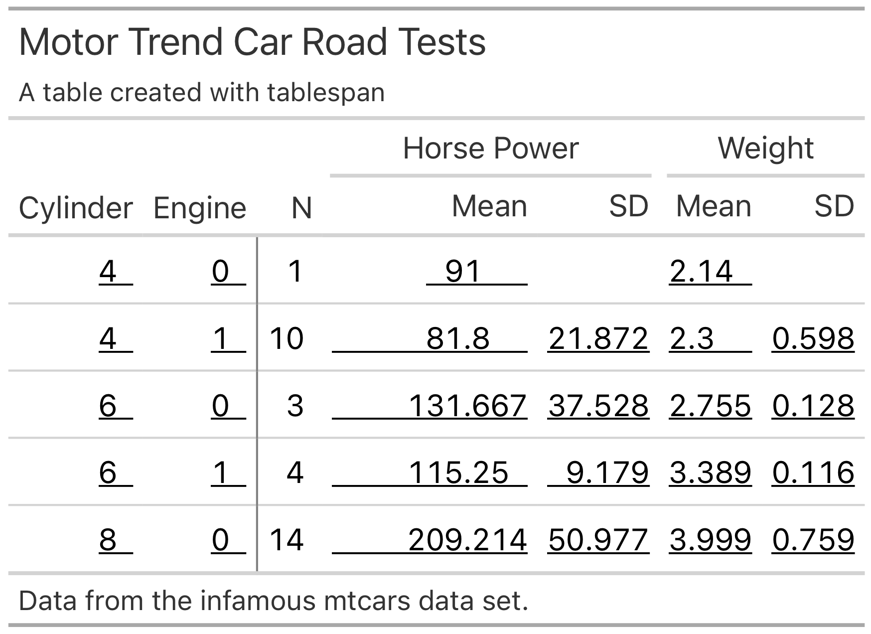
The current interface only exports a small amount of the styles
available in gt and openxlsx. However, you can also provide custom
styles:
tbl |>
  style_column(
    columns = dplyr::where(is.double),
    # custom style for the gt table export:
    gt_style = gt::cell_text(decorate = "underline"),
    # custom style for the excel table export:
    openxlsx_style = openxlsx::createStyle(textDecoration = "underline")
  ) |>
  as_gt()
Formatting
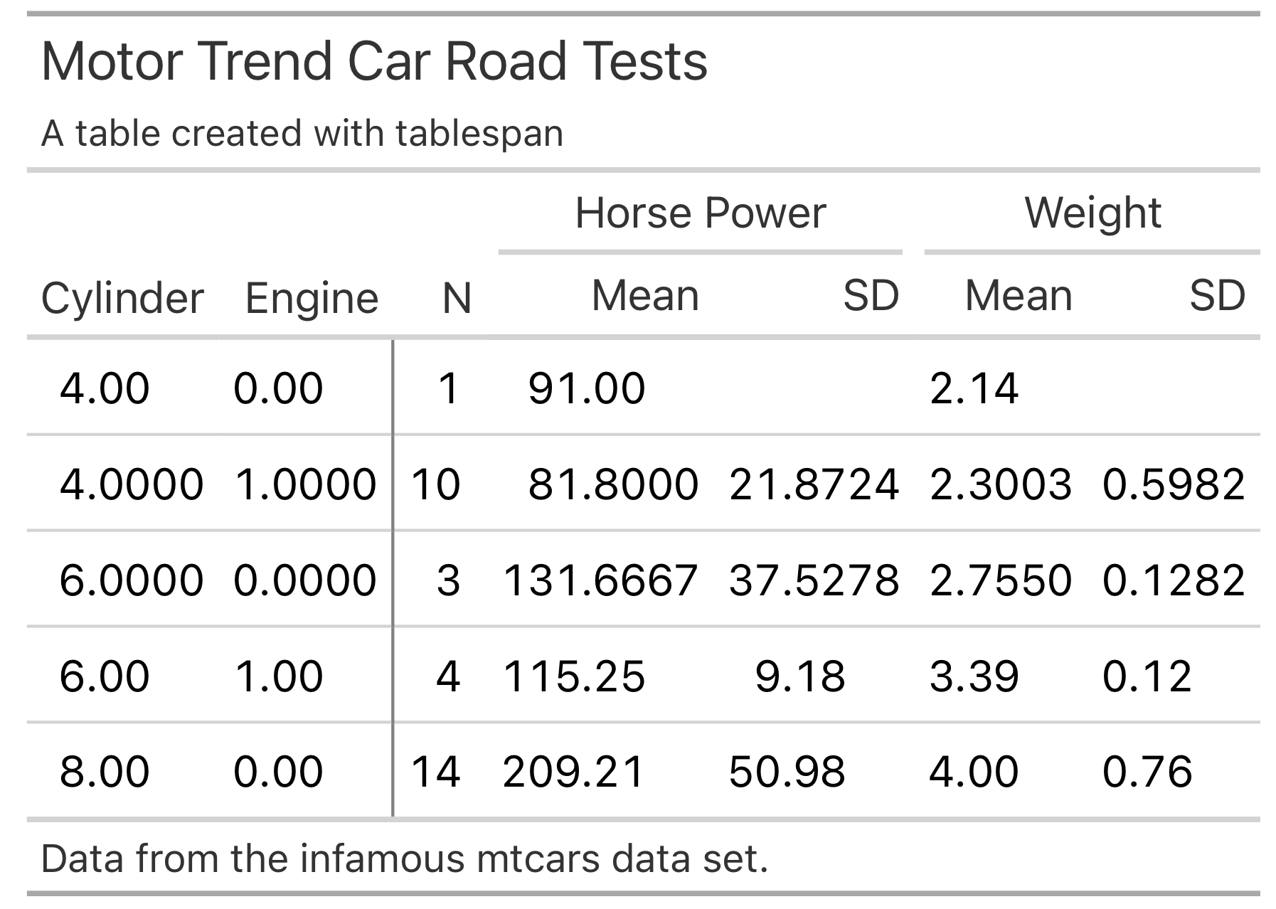
In addition to applying specific styles to the table, you can also adapt
the number formatting. The current setup is slightly more complicated
because unifying all of the possible styles supported by gt and
openxlsx is challenging.
tbl |>
  format_column(
        columns = dplyr::where(is.double),
        rows = 2:3,
        # For great tables, we need a function that
        # takes in the table, columns, and rows and then
        # applies the style
        format_gt = function(x, columns, rows, ...) {
          gt::fmt_number(x, columns = columns, rows = rows, decimals = 4)
        },
        # For openxlsx, we have to provide the style that will be passed
        # to numFmt in openxlsx::createStyle
        format_openxlsx = "0.0000"
      ) |>
  as_gt()
Adapting Great Tables
The gt package provides a wide range of functions to adapt the style
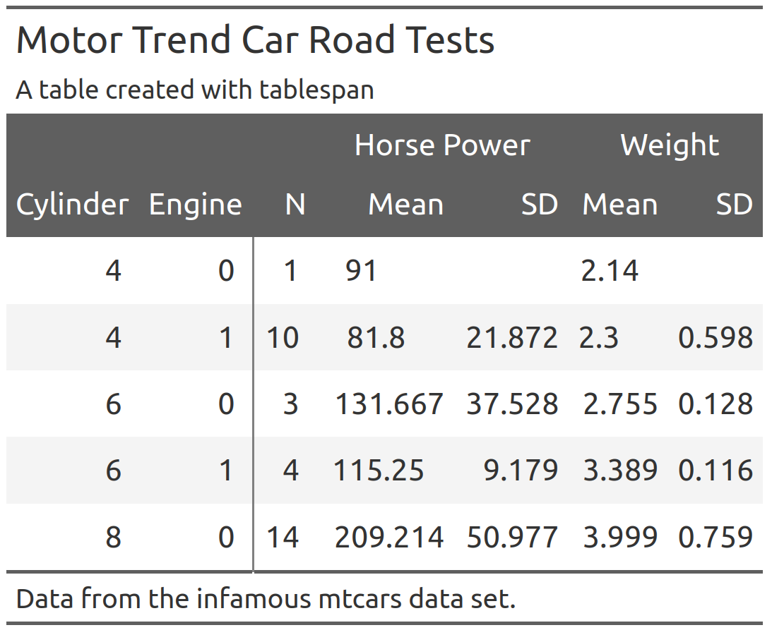
of the table created with as_gt. For instance, opt_stylize adds a
pre-defined style to the entire table:
gt_tbl |>
  gt::opt_stylize(style = 6,
                  color = 'gray')
When adapting the gt object, there is an important detail to keep in
mind: To ensure that each table spanner has a unique ID, tablespan
will create IDs that differ from the text shown in the spanner. To
demonstrate this, Let’s assume that we want to add a spanner above
Horse Power and Weight:
gt_tbl |>
  gt::tab_spanner(label = "New Spanner",
                  spanners = c("Horse Power", "Weight"))
#> Error in `gt::tab_spanner()`:
#> ! One or more spanner ID(s) supplied in `spanners` (Horse Power and
#>   Weight), for the new spanner with the ID `New Spanner` doesn't belong to any
#>   existing spanners.
This will throw an error because the spanner IDs are different from the
spanner labels. To get the spanner IDs, use gt::tab_info():
gt_tbl |>
  gt::tab_info()
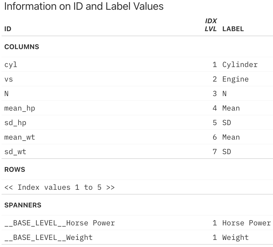
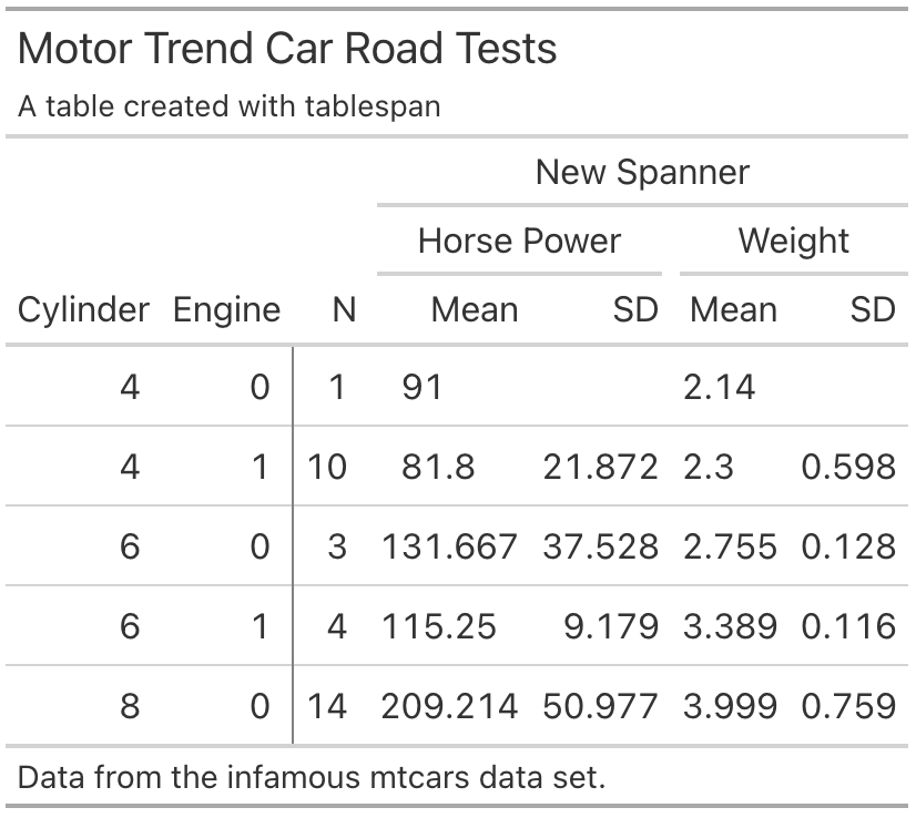
The IDs for the spanners can be found at the very bottom. To add another
spanner above Horse Power and Weight, we have to use these IDs:
gt_tbl |>
  gt::tab_spanner(label = "New Spanner",
                  spanners = c("__BASE_LEVEL__Horse Power",
                               "__BASE_LEVEL__Weight"))
References
- gt: Iannone R, Cheng J, Schloerke B, Hughes E, Lauer A, Seo J, Brevoort K, Roy O (2024). gt: Easily Create Presentation-Ready Display Tables. R package version 0.11.1.9000, https://github.com/rstudio/gt, https://gt.rstudio.com.
- expss: Gregory D et al. (2024). expss: Tables with Labels in R. R package version 0.9.31, https://gdemin.github.io/expss/.
- tables: Murdoch D (2024). tables: Formula-Driven Table Generation. R package version 0.9.31, https://dmurdoch.github.io/tables/.
- openxlsx: Schauberger P, Walker A (2023). openxlsx: Read, Write and Edit xlsx Files. R package version 4.2.5.2, https://ycphs.github.io/openxlsx/.