Stratified Randomized Experiments

Estimate average treatment effects (ATEs) in stratified randomized experiments. 'sreg' supports a wide range of stratification designs, including matched pairs, n-tuple designs, and larger strata with many units — possibly of unequal size across strata. 'sreg' is designed to accommodate scenarios with multiple treatments and cluster-level treatment assignments, and accommodates optimal linear covariate adjustment based on baseline observable characteristics. 'sreg' computes estimators and standard errors based on Bugni, Canay, Shaikh (2018) ; Bugni, Canay, Shaikh, Tabord-Meehan (2024+) ; Jiang, Linton, Tang, Zhang (2023+) ; Bai, Jiang, Romano, Shaikh, and Zhang (2024) ; Bai (2022) ; Bai, Romano, and Shaikh (2022) ; Liu (2024+) ; and Cytrynbaum (2024) .

sreg: Stratified Randomized Experiments

The sreg package for R, offers a toolkit for estimating average treatment effects (ATEs) in stratified randomized experiments. It supports a wide range of stratification designs, including matched pairs, $k$-tuple designs, and larger strata with many units — possibly of unequal size across strata. The package is designed to accommodate scenarios with multiple treatments, and cluster-level treatment assignments, and accomodates optimal linear covariate adjustment based on baseline observable characteristics. The package computes estimators and standard errors based on Bugni, Canay, Shaikh (2018); Bugni, Canay, Shaikh, Tabord-Meehan (2023); Jiang, Linton, Tang, Zhang (2023); Bai, Jiang, Romano, Shaikh, Zhang (2024); Bai (2022); Bai, Romano, Shaikh (2022); Liu (2024); and Cytrynbaum (2024).

Dependencies: dplyr, tidyr, extraDistr, rlang

Suggests: haven, knitr, rmarkdown, testthat (>= 3.0.0)

R version required: >= 2.10

Latest Build (v.2.0.2.9000)

Authors

Juri Trifonov [email protected]
Yuehao Bai [email protected]
Azeem Shaikh [email protected]
Max Tabord-Meehan [email protected]

Supplementary files

PDF version of the manual: Download PDF
Large Strata: Sketch of the derivation of the ATE variance estimator under cluster-level treatment assignment: Download PDF
Large Strata: Expressions for the multiple treatment case (with and without clusters): Download PDF
Small Strata: Expressions for the multiple treatment case (with and without clusters): Download PDF
Mixed Design: Expressions for the multiple treatment case (with and without clusters): Download PDF

Installation

Install the official CRAN release using:

install.packages("sreg")

trying URL 'https://ftp.osuosl.org/pub/cran/src/contrib/sreg_2.0.2.tar.gz'
Content type 'application/x-gzip' length 43389 bytes (42 KB)
==================================================
downloaded 42 KB

* installing *source* package ‘sreg’ ...
** package ‘sreg’ successfully unpacked and MD5 sums checked
** using staged installation
** R
** data
*** moving datasets to lazyload DB
** inst
** byte-compile and prepare package for lazy loading
** help
*** installing help indices
** building package indices
** installing vignettes
** testing if installed package can be loaded from temporary location
** testing if installed package can be loaded from final location
** testing if installed package keeps a record of temporary installation path
* DONE (sreg)

The downloaded source packages are in
        ‘/private/var/folders/mp/06gjwr8j56zdp5j2vgdkd4z40000gq/T/RtmpVk96vN/downloaded_packages’

library(sreg)

#>  ____  ____  _____ ____      Stratified Randomized
#> / ___||  _ \| ____/ ___|     Experiments
#> \___ \| |_) |  _|| |  _  
#>  ___) |  _ <| |__| |_| |  
#> |____/|_| \_\_____\____| version 2.0.2

#> Type 'citation("sreg")' for citing this R package in publications.

The latest development version can be installed using devtools.

library(devtools)
install_github("jutrifonov/sreg")

Downloading GitHub repo jutrifonov/sreg@HEAD
── R CMD build ───────────────────────────────────────────────────────────────────────────────────────────────────────────────────────────────────────────────────────────────────────────────────────────────────────────────────
✔  checking for file ‘/private/var/folders/mp/06gjwr8j56zdp5j2vgdkd4z40000gq/T/RtmpVk96vN/remotes1026130d7f9b4/jutrifonov-sreg-53c1377/DESCRIPTION’ ...
─  preparing ‘sreg’:
✔  checking DESCRIPTION meta-information ..
─  checking for LF line-endings in source and make files and shell scripts
─  checking for empty or unneeded directories
─  building ‘sreg_2.0.2.tar.gz’
   
Installing package into ‘/opt/homebrew/lib/R/4.4/site-library’
(as ‘lib’ is unspecified)
* installing *source* package ‘sreg’ ...
** using staged installation
** R
** data
*** moving datasets to lazyload DB
** inst
** byte-compile and prepare package for lazy loading
** help
*** installing help indices
** building package indices
** installing vignettes
** testing if installed package can be loaded from temporary location
** testing if installed package can be loaded from final location
** testing if installed package keeps a record of temporary installation path
* DONE (sreg)

library(sreg)

ℹ Loading sreg
#>  ____  ____  _____ ____      Stratified Randomized
#> / ___||  _ \| ____/ ___|     Experiments
#> \___ \| |_) |  _|| |  _  
#>  ___) |  _ <| |__| |_| |  
#> |____/|_| \_\_____\____| version 2.0.2
                           

#> Type 'citation("sreg")' for citing this R package in publications.

Function: `sreg()`

Estimates the ATE(s) and the corresponding standard error(s) for a (collection of) treatment(s) relative to a control.

Syntax

sreg(Y, S = NULL, D, G.id = NULL, Ng = NULL, X = NULL,
     HC1 = TRUE, small.strata = FALSE, k = NULL)

Arguments

Y - a numeric vector/matrix/data.frame/tibble of the observed outcomes;
S - a numeric vector/matrix/data.frame/tibble of strata indicators $\{0, 1, 2, \ldots\}$; if NULL then the estimation is performed assuming no stratification;
D - a numeric vector/matrix/data.frame/tibble of treatments indexed by $\{0, 1, 2, \ldots\}$, where D = 0 denotes the control;
G.id - a numeric vector/matrix/data.frame/tibble of cluster indicators; if NULL then estimation is performed assuming treatment is assigned at the individual level;
Ng - a numeric vector/matrix/data.frame/tibble of cluster sizes; if NULL then Ng is assumed to be equal to the number of available observations in every cluster;
X - a matrix/data.frame/tibble with columns representing the covariate values for every observation; if NULL then the estimator without linear adjustments is applied [^*];
HC1 - a TRUE/FALSE logical argument indicating whether the small sample correction should be applied to the variance estimator;
small.strata - a TRUE/FALSE logical argument indicating whether the estimators for small strata (i.e., strata with few units, such as matched pairs or n-tuples) should be used [^**];
k - an optional positive integer giving the number of units per small stratum, or the number of clusters per small stratum in a cluster-randomized design. For a uniform small-strata design, k can be omitted because the common size is observed directly. For a mixed design, supply k to identify the small component when it consists of 4-tuples or larger. [^*]: Note: sreg cannot use individual-level covariates for covariate adjustment in cluster-randomized experiments. Any individual-level covariates will be aggregated to their cluster-level averages. [^**]: For a mixed design, at least 25% of the strata must share the size selected for the small component. The threshold concerns strata, not observations. With k = NULL, the package automatically detects conventional pairs and triplets; use an explicit k for general k-tuple mixed designs. The mixed estimator combines the small- and large-strata estimators using observation-count weights. See the supplementary PDF for details and expressions.

Data Structure

Here we provide an example of a data frame that can be used with sreg.

|       Y      | S | D | G.id | Ng |     x_1    |      x_2      |
|--------------|---|---|------|----|------------|---------------|
| -0.57773576  | 2 | 0 |  1   | 10 |  1.5597899 |  0.03023334   |
|  1.69495638  | 2 | 0 |  1   | 10 |  1.5597899 |  0.03023334   |
|  2.02033740  | 4 | 2 |  2   | 30 |  0.8747419 | -0.77090031   |
|  1.22020493  | 4 | 2 |  2   | 30 |  0.8747419 | -0.77090031   |
|  1.64466086  | 4 | 2 |  2   | 30 |  0.8747419 | -0.77090031   |
| -0.32365109  | 4 | 2 |  2   | 30 |  0.8747419 | -0.77090031   |
|  2.21008191  | 4 | 2 |  2   | 30 |  0.8747419 | -0.77090031   |
| -2.25064316  | 4 | 2 |  2   | 30 |  0.8747419 | -0.77090031   |
|  0.37962312  | 4 | 2 |  2   | 30 |  0.8747419 | -0.77090031   |

Summary

sreg prints a "Stata-style" table containing the ATE estimates, corresponding standard errors, $t$-statistics, $p$-values, $95$% asymptotic confidence intervals, and significance indicators for different levels $\alpha$. The example of the printed output is provided below.

Saturated Model Estimation Results under CAR
Observations: 2710 
Clusters: 100 
Number of treatments: 2 
Number of strata: 10 
Setup: large strata
Standard errors: adjusted (HC1) 
Treatment assignment: cluster level 
Covariates used in linear adjustments: 
---
Coefficients:
      Tau   As.se  T-stat P-value CI.left(95%) CI.right(95%) Significance
1 1.13687 0.31181 3.64608 0.00027      0.52574       1.74799          ***
2 0.66447 0.30263 2.19565 0.02812      0.07133       1.25761            *
---
Signif. codes:  0 `***` 0.001 `**` 0.01 `*` 0.05 `.` 0.1 ` ` 1

Return Value

The function returns an object of class sreg that is a list containing the following elements:

tau.hat - a $1 \times |\mathcal A|$ vector of ATE estimates, where $|\mathcal A|$ represents the number of treatments;
se.rob - a $1 \times |\mathcal A|$ vector of standard errors estimates, where $|\mathcal A|$ represents the number of treatments;
t.stat - a $1 \times |\mathcal A|$ vector of $t$-statistics, where $|\mathcal A|$ represents the number of treatments;
p.value - a $1 \times |\mathcal A|$ vector of corresponding $p$-values, where $|\mathcal A|$ represents the number of treatments;
CI.left - a $1 \times |\mathcal A|$ vector of the left bounds of the $95$% as. confidence interval;
CI.right - a $1 \times |\mathcal A|$ vector of the right bounds of the $95$% as. confidence interval;
data - an original data of the form data.frame(Y, S, D, G.id, Ng, X);
lin.adj - a data.frame representing the covariates that were used in implementing linear adjustments;
small.strata - a TRUE/FALSE logical argument indicating whether the estimators for small strata (e.g., matched pairs or n-tuples) were used;
HC1 - a TRUE/FALSE logical argument indicating whether the small sample correction (HC1) was applied to the variance estimator.

Empirical Example

Here, we provide the empirical application example using the data from (Chong et al., 2016), who studied the effect of iron deficiency anemia on school-age children's educational attainment and cognitive ability in Peru. The example replicates the empirical illustration from (Bugni et al., 2019). For replication purposes, the data is included in the package and can be accessed by running data("AEJapp"). This example can be accessed directly in R via help(sreg).

library(sreg, dplyr, haven)

The description of the dataset can be accessed using help():

help(AEJapp)

We can upload the AEJapp dataset to the R session via data():

data("AEJapp")
data <- AEJapp

It is pretty straightforward to prepare the data to fit the package syntax using dplyr:

Y <- data$gradesq34
D <- data$treatment
S <- data$class_level
data.clean <- data.frame(Y, D, S)
data.clean <- data.clean %>%
  mutate(D = ifelse(D == 3, 0, D))
Y <- data.clean$Y
D <- data.clean$D
S <- data.clean$S
head(data.clean)
     Y D S
1 11.2 1 1
2 12.4 0 3
3 11.9 0 5
4 13.1 0 1
5 13.4 2 2
6 10.7 0 1

We can take a look at the frequency table of D and S:

table(D = data.clean$D, S = data.clean$S)
   S
D    1  2  3  4  5
  0 15 19 16 12 10
  1 16 19 15 10 10
  2 17 20 15 11 10

Now, it is straightforward to replicate the results from (Bugni et al, 2019) using sreg:

result <- sreg::sreg(Y = Y, S = S, D = D)
print(result)

Saturated Model Estimation Results under CAR
Observations: 215 
Number of treatments: 2 
Number of strata: 5 
Setup: large strata
Standard errors: adjusted (HC1) 
Treatment assignment: individual level 
Covariates used in linear adjustments: 
---
Coefficients:
       Tau   As.se   T-stat P-value CI.left(95%) CI.right(95%) Significance
1 -0.05113 0.20645 -0.24766 0.80440     -0.45577       0.35351             
2  0.40903 0.20651  1.98065 0.04763      0.00427       0.81379            *
---
Signif. codes:  0 `***` 0.001 `**` 0.01 `*` 0.05 `.` 0.1 ` ` 1

Besides that, sreg allows adding linear adjustments (covariates) to the estimation procedure:

pills <- data$pills_taken
age <- data$age_months
data.clean <- data.frame(Y, D, S, pills, age)
data.clean <- data.clean %>%
  mutate(D = ifelse(D == 3, 0, D))
Y <- data.clean$Y
D <- data.clean$D
S <- data.clean$S
X <- data.frame("pills" = data.clean$pills, "age" = data.clean$age)
result <- sreg::sreg(Y, S, D, G.id = NULL, X = X)
print(result)
Saturated Model Estimation Results under CAR with linear adjustments
Observations: 215 
Number of treatments: 2 
Number of strata: 5 
Setup: large strata
Standard errors: adjusted (HC1) 
Treatment assignment: individual level 
Covariates used in linear adjustments: pills, age
---
Coefficients:
       Tau   As.se   T-stat P-value CI.left(95%) CI.right(95%) Significance
1 -0.02862 0.17964 -0.15929 0.87344     -0.38071       0.32348             
2  0.34609 0.18362  1.88477 0.05946     -0.01381       0.70598            .
---
Signif. codes:  0 `***` 0.001 `**` 0.01 `*` 0.05 `.` 0.1 ` ` 1

Example (small strata)

Beginning with version 2.0.0+, the sreg package supports experimental designs with small strata (e.g., matched pairs or k-tuples) via the small.strata argument in the sreg function. We demonstrate its implementation using simulated data generated by sreg.rgen() under a matched triplets design.

data <- sreg.rgen(n = 300, tau.vec = c(1.2, 0.8), cluster = FALSE, small.strata = TRUE, k = 3, treat.sizes = c(1, 1, 1))
> head(data)

           Y S D      x_1       x_2
1  2.6455170 1 0 5.594675 1.9023835
2  6.6589024 1 2 6.450984 4.2343208
3  4.3412644 1 1 4.787852 3.1895694
4 -0.7592291 2 2 6.240883 0.7458935
5  5.1391241 2 1 6.076305 2.6105942
6  2.3934378 2 0 5.403182 3.4032419

result <- sreg(Y = data$Y, S = data$S, D = data$D, X = data.frame('x_1' = data$x_1, 'x_2' = data$x_2), small.strata = TRUE)
> print(result)
Saturated Model Estimation Results under CAR with linear adjustments
Observations: 300 
Number of treatments: 2 
Number of strata: 100 
Setup: small strata 
Strata size (k): 3 
Standard errors: adjusted (HC1) 
Treatment assignment: individual level 
Covariates used in linear adjustments: x_1, x_2
---
Coefficients:
      Tau   As.se  T-stat P-value CI.left(95%) CI.right(95%) Significance
1 1.11577 0.13995 7.97258   0e+00      0.84147       1.39006          ***
2 0.58806 0.13439 4.37574   1e-05      0.32466       0.85147          ***
---
Signif. codes:  0 `***` 0.001 `**` 0.01 `*` 0.05 `.` 0.1 ` ` 1

Because all strata in this example have the same size, sreg() observes k = 3 directly. Supplying k = 3 to sreg() is optional and acts as a validation check.

Example (mixed small and large strata)

Set mixed.strata = TRUE in sreg.rgen() to generate both components in one call. Here, 80 observations form 20 small strata of size four, and the remaining 40 observations form four large strata:

mixed_data <- sreg.rgen(
  n = 120,
  tau.vec = 0.5,
  cluster = FALSE,
  mixed.strata = TRUE,
  n.small = 80,
  k = 4,
  treat.sizes = c(2, 2),
  n.strata = 4
)

mixed_fit <- sreg(
  Y = mixed_data$Y,
  S = mixed_data$S,
  D = mixed_data$D,
  small.strata = TRUE,
  k = 4
)

For mixed designs, k identifies the intended small-stratum size. If it is omitted, sreg() retains automatic detection for matched pairs and triplets. An explicit value is therefore required for mixed 4-tuples and larger k-tuples. At least 25% of all strata must have the specified size; otherwise, the function returns an error rather than guessing another k.

S3 Method: `plot.sreg()`

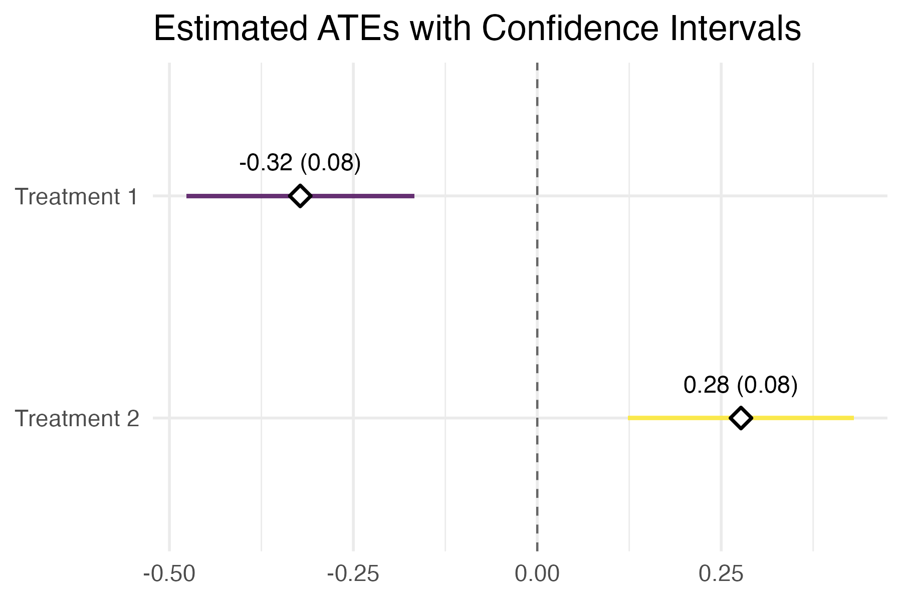
Visualizes the estimated average treatment effects (ATEs) and their confidence intervals from an object returned by sreg(). This function defines an S3 method for the generic plot() function for objects of class sreg.

Syntax

plot(x,
     treatment_labels = NULL,
     title = "Estimated ATEs with Confidence Intervals",
     bar_fill = NULL,
     point_shape = 23,
     point_size = 3,
     point_fill = "white",
     point_stroke = 1.2,
     point_color = "black",
     label_color = "black",
     label_size = 4,
     bg_color = NULL,
     grid = TRUE,
     zero_line = TRUE,
     y_axis_title = NULL,
     x_axis_title = NULL,
     ...)

Arguments

x - an object of class sreg, returned by the sreg() function;
treatment_labels - an optional vector of labels to display on the y-axis; if NULL, defaults to "Treatment 1", "Treatment 2", etc.;
title - an optional string specifying the plot title; default is "Estimated ATEs with Confidence Intervals";
bar_fill - an optional color specification for the confidence interval bars; can be NULL (default viridis scale), a single color, or a vector of two colors for a gradient;
point_shape - an integer specifying the shape of the point representing the estimated ATE; default is 23 (diamond);
point_size - a numeric value specifying the size of the ATE point;
point_fill - a string indicating the fill color of the ATE point shape;
point_stroke - a numeric value for the stroke (border thickness) of the ATE point shape;
point_color - a string specifying the outline color of the ATE point;
label_color - a string indicating the color of the text label displaying the estimate and standard error;
label_size - a numeric value for the size of the text label;
bg_color - an optional string specifying the background color of the plot panel; if NULL, the default theme background is used;
grid - a TRUE/FALSE argument indicating whether grid lines should be displayed (TRUE by default);
zero_line - a TRUE/FALSE argument indicating whether to include a dashed vertical line at 0 (TRUE by default);
y_axis_title - an optional string specifying the y-axis title; if NULL, no title is displayed;
x_axis_title - an optional string specifying the x-axis title; if NULL, no title is displayed;
... - additional arguments passed to other methods (not used in this method).

Return Value

Invisibly returns the ggplot object used to generate the figure. The function is called primarily for its side effect — rendering the plot.

Example

library("sreg")
library("dplyr")
library("haven")
data <- sreg.rgen(n = 1000, tau.vec = c(-0.3, 0.2), n.strata = 4, cluster = FALSE)
Y <- data$Y
S <- data$S
D <- data$D
X <- data.frame("x_1" = data$x_1, "x_2" = data$x_2)
result <- sreg(Y, S, D, G.id = NULL, Ng = NULL, X)
plot(result)

Example Plot

S3 Method: `print.sreg()`

Prints a summary table of the estimated treatment effects from an object returned by sreg(). This function defines an S3 method for the generic print() function for objects of class sreg. This method prints a formatted summary table that includes the estimated average treatment effects, standard errors, $p$-values, confidence intervals, and details about the experimental design.

Syntax

print.sreg(x, ...)

Arguments

x - an object of class sreg, typically returned by the sreg() function;
... - additional arguments.

Function `sreg.rgen()`

Generates the observed outcomes, treatment assignments, strata indicators, cluster indicators, cluster sizes, and covariates for estimating the treatment effect following the stratified block randomization design under covariate-adaptive randomization (CAR).

Syntax

sreg.rgen(n, Nmax = 50, n.strata = 10,
         tau.vec = c(0), gamma.vec = c(0.4, 0.2, 1),
         cluster = TRUE, is.cov = TRUE, small.strata = FALSE,
         k = 3, treat.sizes = c(1, 1, 1),
         mixed.strata = FALSE, n.small = NULL)

Arguments

n - the total number of units when cluster = FALSE, or the total number of clusters when cluster = TRUE;
Nmax - a maximum size of generated clusters (maximum number of observations in a cluster);
n.strata - an integer specifying the number of strata;
tau.vec - a numeric $1 \times |\mathcal A|$ vector of treatment effects, where $|\mathcal A|$ represents the number of treatments;
gamma.vec - a numeric $1 \times 3$ vector of parameters corresponding to covariates;
cluster - a TRUE/FALSE argument indicating whether the dgp should use a cluster-level treatment assignment or individual-level;
is.cov - a TRUE/FALSE argument indicating whether the dgp should include covariates or not;
small.strata - a TRUE/FALSE argument indicating whether the data-generating process should use a small-strata design (e.g., matched pairs, $n$-tuples);
k - an integer specifying the number of units per stratum when small.strata = TRUE;
treat.sizes - a numeric $1 \times (|\mathcal A| + 1)$ vector specifying the number of units assigned to each treatment within a stratum; the first element corresponds to control units ($D = 0$), the second to the first treatment ($D = 1$), and so on.
mixed.strata - a TRUE/FALSE argument indicating whether to generate both small and large strata;
n.small - the number of units, or clusters for cluster-randomized designs, assigned to the small-strata component. It must be divisible by k. If NULL, the largest multiple of k not exceeding half of n is used.

Return Value

Y - a numeric $n \times 1$ vector of the observed outcomes;
S - a numeric $n \times 1$ vector of strata indicators;
D - a numeric $n \times 1$ vector of treatments indexed by $\{0, 1, 2, \ldots\}$, where D = 0 denotes the control;
G.id - a numeric $n \times 1$ vector of cluster indicators;
Ng - a numeric vector/matrix/data.frame of cluster sizes; if NULL then Ng is assumed to be equal to the number of available observations in every cluster;
X - a data.frame with columns representing the covariate values for every observation.

Example

library(sreg)
# big stata
data <- sreg.rgen(n = 1000, tau.vec = c(0), n.strata = 4, cluster = TRUE)
> head(data)
         Y S D      x_1       x_2
1 1.717293 1 0 4.772092 2.4138491
2 2.553695 2 0 5.413440 2.0551019
3 2.237556 3 2 6.611161 0.9300293
4 1.825809 3 1 2.735503 1.7839981
5 5.536280 2 2 2.469239 2.0495611
6 1.628753 2 0 4.887561 2.1327071

# matched pairs (small strata)
data <- sreg.rgen(n = 100, tau.vec = c(1.2), cluster = FALSE, small.strata = TRUE, k = 2, treat.sizes = c(1, 1))
> head(data)
          Y S D      x_1      x_2
1 2.0393535 1 1 7.904694 1.487941
2 3.3839515 1 0 3.461776 2.832059
3 1.7250989 2 0 3.049906 3.170014
4 3.0991776 2 1 7.437064 1.098371
5 1.7406104 3 1 5.008703 1.750753
6 0.6986514 3 0 3.418835 1.375744

# mixed design with 4-tuples and large strata
mixed_data <- sreg.rgen(
  n = 120, tau.vec = 0.5, cluster = FALSE,
  mixed.strata = TRUE, n.small = 80, k = 4,
  treat.sizes = c(2, 2), n.strata = 4
)

References

Bugni, F. A., Canay, I. A., and Shaikh, A. M. (2018). Inference Under Covariate-Adaptive Randomization. Journal of the American Statistical Association, 113(524), 1784–1796, doi:10.1080/01621459.2017.1375934.

Bugni, F., Canay, I., Shaikh, A., and Tabord-Meehan, M. (2024+). Inference for Cluster Randomized Experiments with Non-ignorable Cluster Sizes. Forthcoming in the Journal of Political Economy: Microeconomics, doi:10.48550/arXiv.2204.08356.

Jiang, L., Linton, O. B., Tang, H., and Zhang, Y. (2023+). Improving Estimation Efficiency via Regression-Adjustment in Covariate-Adaptive Randomizations with Imperfect Compliance. Forthcoming in Review of Economics and Statistics, doi:10.48550/arXiv.2204.08356.

Bai, Y., Jiang, L., Romano, J. P., Shaikh, A. M., and Zhang, Y. (2024). Covariate adjustment in experiments with matched pairs. Journal of Econometrics, 241(1), doi:10.1016/j.jeconom.2024.105740.

Bai, Y. (2022). Optimality of Matched-Pair Designs in Randomized Controlled Trials. American Economic Review, 112(12), doi:10.1257/aer.20201856.

Bai, Y., Romano, J. P., and Shaikh, A. M. (2022). Inference in Experiments With Matched Pairs. Journal of the American Statistical Association, 117(540), doi:10.1080/01621459.2021.1883437.

Liu, J. (2024). Inference for Two-stage Experiments under Covariate-Adaptive Randomization. doi:10.48550/arXiv.2301.09016.

Cytrynbaum, M. (2024). Covariate Adjustment in Stratified Experiments. Quantitative Economics, 15(4), 971–998, doi:10.3982/QE2475

Reference manual

install.packages("sreg")

2.1.0 by Juri Trifonov, 2 months ago

https://github.com/jutrifonov/sreg

Report a bug at https://github.com/jutrifonov/sreg/issues

Browse source code at https://github.com/cran/sreg

Authors: Juri Trifonov [aut, cre, cph] , Yuehao Bai [aut] , Azeem Shaikh [aut] , Max Tabord-Meehan [aut]

Documentation: PDF Manual

MIT + file LICENSE license

Imports dplyr, tidyr, purrr, extraDistr, rlang, cli, ggplot2, viridis

Suggests haven, knitr, rmarkdown, testthat

See at CRAN

sreg

Stratified Randomized Experiments

sreg: Stratified Randomized Experiments

Authors

Supplementary files

Installation

Function: sreg()

Syntax

Arguments

Data Structure

Summary

Return Value

Empirical Example

Example (small strata)

Example (mixed small and large strata)

S3 Method: plot.sreg()

Syntax

Arguments

Return Value

Example

S3 Method: print.sreg()

Syntax

Arguments

Function sreg.rgen()

Syntax

Arguments

Return Value

Example

References

Reference manual

R links

R homepage

Download R

Mailing lists

R documentation

R manuals

R FAQs

The R Journal

CRAN links

CRAN homepage

CRAN repository policy

Submit a package

METACRAN stuff

About METACRAN

At github

Report a bug

Function: `sreg()`

S3 Method: `plot.sreg()`

S3 Method: `print.sreg()`

Function `sreg.rgen()`