Create Graphics of 'R' Data Structures

Draws teaching diagrams of the contents of common 'R' data structures (vectors, matrices, data frames, lists, and arrays) so their shape and values can be read at a glance. Two backends render the same picture, with base 'R' graphics through the paint_*() functions and 'ggplot2' through the gpaint_*() functions. The label under each cell is the expression you would type to reach that cell, so every diagram doubles as a lesson in how to subset and index the object it draws.

paintr

The goal of paintr is to draw different R data structures as pictures. Each value sits in its own cell, and under each cell paintr writes the expression you would type to reach it – so the drawing and the code are the same object. It is built for teaching, where the hard part is helping someone see the shape of the thing they are working with.

[!NOTE]

A previous version of the package was called drawr; however, another package with the same name was published on CRAN. As a result, the package was renamed to paintr.

Installation

You can install the development version of paintr from GitHub with:

# install.packages("remotes")
remotes::install_github("coatless-rpkg/paintr")

Design

The package takes advantage of base R graphics alongside ggplot2. Every structure has two painters, under the naming scheme:

paint_*(): base R graphics, drawn straight to the device.
gpaint_*(): ggplot2, returning a ggplot object you can print or save.

paintr draws five structures: vectors, matrices, data frames, lists, and arrays.

library(paintr)

Vectors

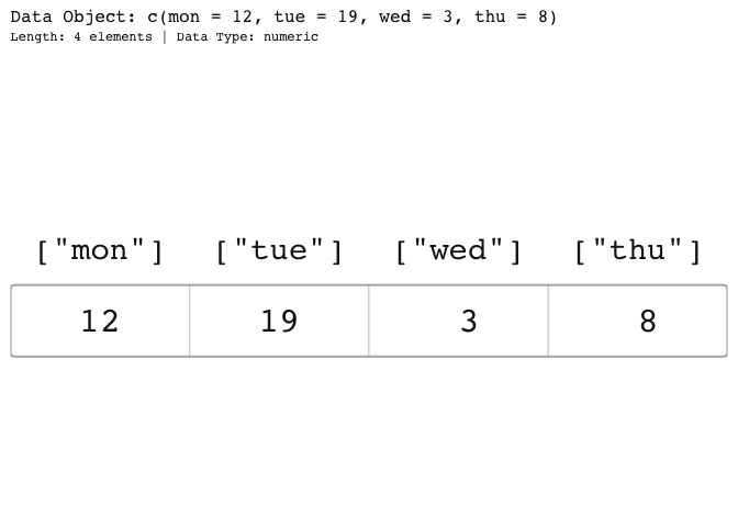
A vector is a one-dimensional run of values, and that is how it draws. Under each cell is the expression you would type to reach it: [3] for the third value. Give the vector names and the label becomes the named accessor, ["mon"], because x["mon"] is now how you reach that value.

paint_vector(c(mon = 12, tue = 19, wed = 3, thu = 8), layout = "horizontal")

A named numeric vector shown as one horizontal row of four cells holding 12, 19, 3, and 8, with the named accessor label for each day written under its cell: mon, tue, wed, and thu.

Matrices

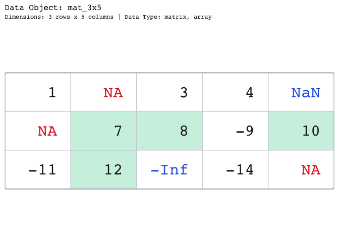
A matrix is a grid, so it draws as one. Take a matrix with a few awkward values:

mat_3x5 = matrix(
  c(
   1, NA,    3,   4,  NaN,
  NA,  7,    8,  -9,  10,
 -11, 12, -Inf, -14,  NA
 ),
 ncol = 5, byrow = TRUE)

mat_3x5
#>      [,1] [,2] [,3] [,4] [,5]
#> [1,]    1   NA    3    4  NaN
#> [2,]   NA    7    8   -9   10
#> [3,]  -11   12 -Inf  -14   NA

We can lay out its contents, label the cells with their [row, column] subscript, or highlight the cells that meet a condition – a comparison is a highlight mask.

# Show the cell indices
paint_matrix(mat_3x5, show_indices = "cell")

A 3 by 5 matrix shown as a grid of cells holding its values, including NA, NaN, and -Inf, with each cell labeled below by its [row, column] subscript.

# Highlight cells over a specific value
paint_matrix(mat_3x5, highlight_area = mat_3x5 > 4)

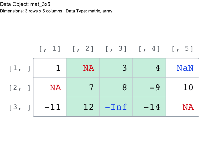
The same 3 by 5 matrix grid with the cells whose value exceeds 4 highlighted, using the comparison mat_3x5 greater than 4 as a highlight mask.

The same picture is available with ggplot2:

gpaint_matrix(mat_3x5,
             show_indices = c("row", "column"),
             highlight_area = highlight_columns(mat_3x5, columns = 2:4))

A ggplot2 rendering of the same 3 by 5 matrix, with row indices in a left gutter and column indices along the top, and columns 2 through 4 highlighted.

Data frames

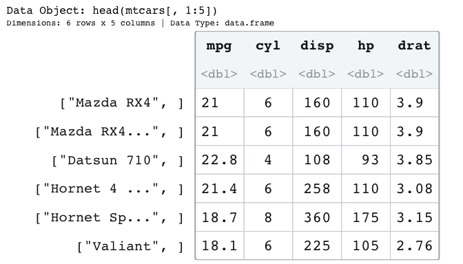
A data frame gets the richest default picture: a header of column names, the type of each column beneath it, and a row-name gutter when the row names are meaningful. Numbers show three significant figures, with trailing digits in grey.

paint_data_frame(head(mtcars[, 1:5]))

The first six rows of the first five columns of mtcars drawn as a data frame: a header of column names, the type of each column beneath it, a row-name gutter, and numeric values shown to three significant figures.

Lists

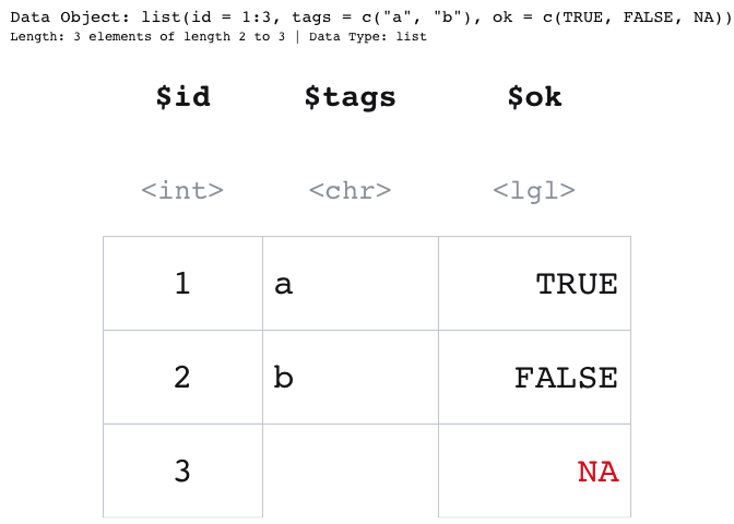
A list is the flexible container: its elements can differ in length and type, so paintr draws each element as a column. A data frame is just a list whose elements share a length – break one length and the rectangle breaks with it.

paint_list(list(id = 1:3, tags = c("a", "b"), ok = c(TRUE, FALSE, NA)))

A list drawn with each element as its own column: id holding 1, 2, and 3; tags holding the strings a and b; and ok holding TRUE, FALSE, and NA, so the columns differ in length and type.

Arrays

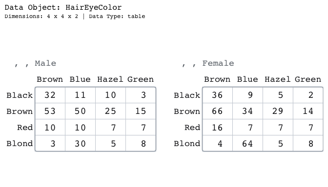
An array of three or more dimensions is a stack of matrices, and paint_array() lays that stack out as a row of blocks sharing one font size. The label under a cell is its full subscript, a genuine n-dimensional index.

paint_array(HairEyeColor)

The HairEyeColor array drawn as a row of matrix blocks sharing one font size, one block per layer of the third dimension, with each cell labeled below by its full n-dimensional subscript.

Learn more

Four vignettes go deeper:

Getting started with paintr – the full tour of all five structures.
Highlighting cells – spotlight rows, columns, and individual cells.
Base graphics and ggplot2 – the paint_ and gpaint_ split, and when each backend pays off.
Teaching with paintr – putting these pictures to work in lessons.