ozbabynames
Australian Popular Baby Names
Data on the most popular baby names by sex and year, and for each state in Australia, as provided by the state and territory governments. The quality and quantity of the data varies with the state.
ozbabynames 
The ozbabynames package provides the dataset ozbabynames. This
contains popular Australian baby names by sex, state and year.
library(ozbabynames)
head(ozbabynames)
#>   year           state    sex      name count
#> 1 2024 New South Wales Female Charlotte   383
#> 2 2024 New South Wales Female    Amelia   367
#> 3 2024 New South Wales Female    Olivia   316
#> 4 2024 New South Wales Female       Mia   308
#> 5 2024 New South Wales Female      Isla   298
#> 6 2024 New South Wales Female     Chloe   275
Installation
You can install the development version of ozbabynames from github:
install_github("robjhyndman/ozbabynames")
The CRAN version can be installed using:
install.packages("ozbabynames")
Related packages
- babynames - US baby names from 1880 to 2017.
- nzbabynames - New Zealand baby names from 1900 to 2017.
- norwaynames - Norway baby names from 1880 to 2017.
Related data
Example usage
library(ggplot2)
library(dplyr)

ozbabynames_1952_top_10 <- ozbabynames |>
  filter(year == 1952) |>
  group_by(sex, name) |>
  summarise(count = sum(count)) |>
  arrange(-count) |>
  top_n(10) |>
  ungroup()

ggplot(
  ozbabynames_1952_top_10,
  aes(
    x = reorder(name, count),
    y = count,
    group = sex
  )
) +
  geom_col() +
  facet_grid(sex ~ .,
    scales = "free_y"
  ) +
  coord_flip() +
  ylab("Count") +
  xlab("Name") +
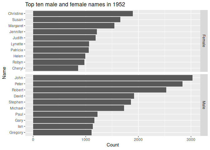
  ggtitle("Top ten male and female names in 1952")
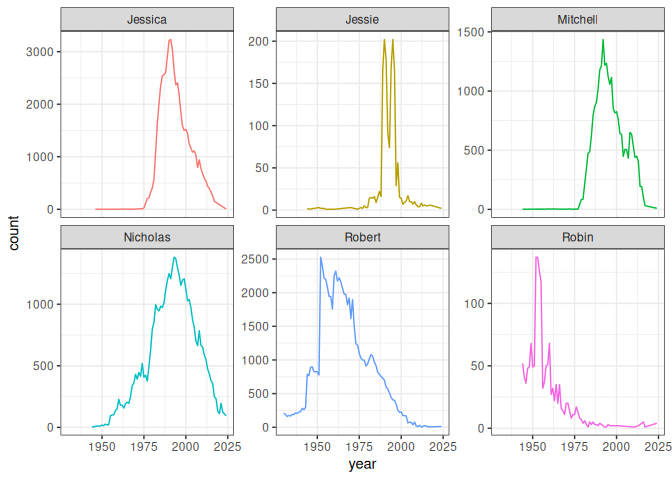
And let’s look at the popularity of the package author names, “Rob”, “Mitchell”, “Nicholas”, and “Jessie”, as well as some similar names.
author_names <- c("Robin", "Robert", "Mitchell", "Nicholas", "Jessie", "Jessica")

ozbabynames |>
  filter(name %in% author_names) |>
  group_by(name, year) |>
  summarise(count = sum(count)) |>
  ggplot(aes(
    x = year,
    y = count,
    colour = name
  )) +
  geom_line() +
  theme_bw() +
  facet_wrap(~name,
    scales = "free_y"
  ) +
  theme(legend.position = "none")
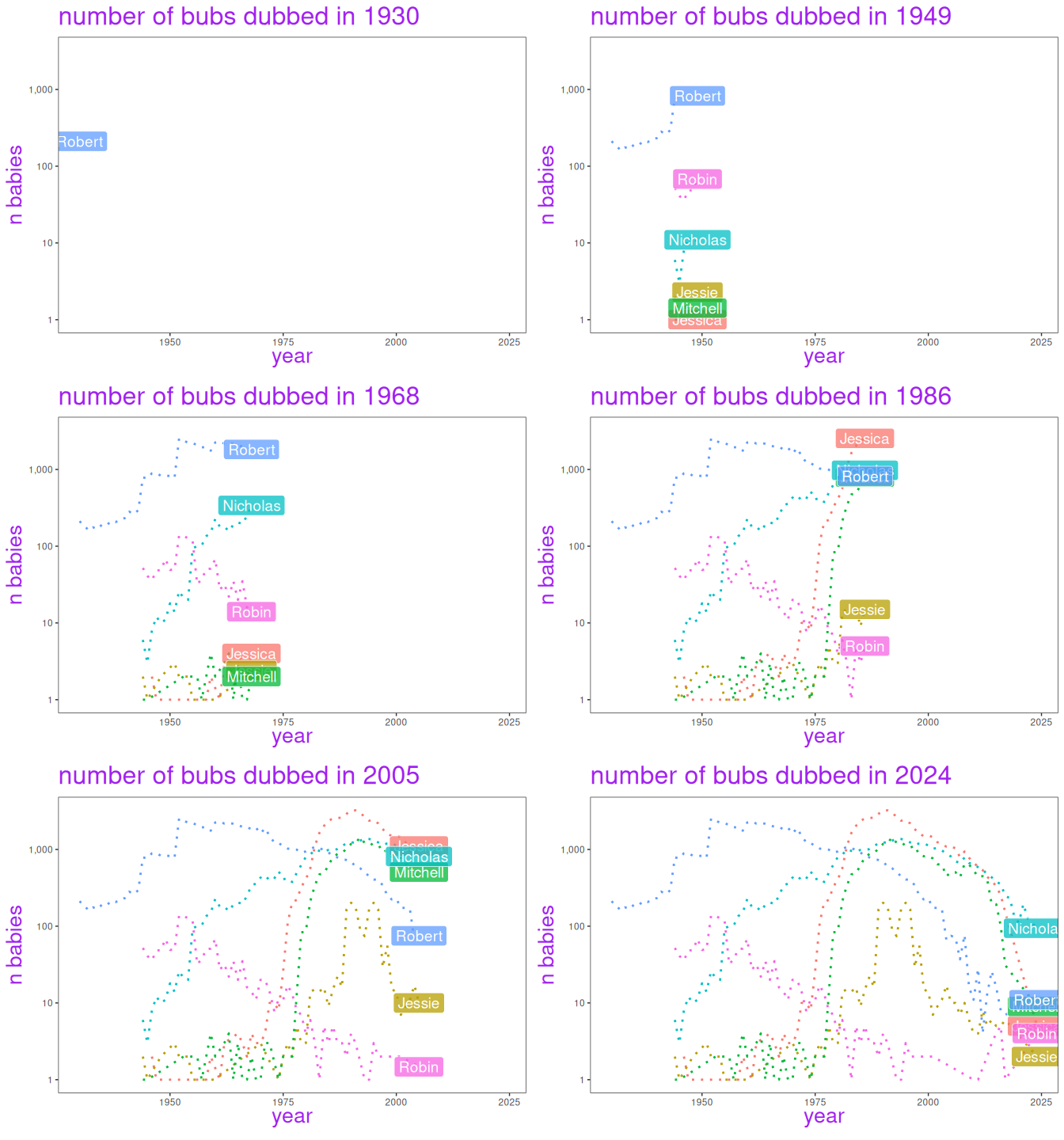
And let’s see that animated
library(gganimate)

ozbabynames |>
  filter(name %in% author_names) |>
  count(name, year, wt = count) |>
  ggplot(aes(
    x = year,
    y = n,
    colour = name,
    group = name,
    label = name,
    fill = name
  )) +
  geom_line(linewidth = 1, linetype = "dotted") +
  geom_label(colour = "white", alpha = 0.75, size = 5) +
  theme_bw() +
  theme(
    panel.grid = element_blank(),
    legend.position = "none",
    title = element_text(
      colour = "purple",
      size = 20,
      face = "bold"
    )
  ) +
  labs(
    title = "number of bubs dubbed in {frame_along} ",
    y = "n babies"
  ) +
  scale_y_log10(labels = scales::comma) +
  transition_reveal(along = year)
Known Issues
The coverage is very uneven, with some states only providing very recent data, and some states only providing the top 50 or 100 names. The ACT does not provide counts, and so no ACT data are included. South Australia has by far the best data, with full coverage of all names back to 1944.
Sources
-
Tasmania