miclust
Multiple Imputation in Cluster Analysis
Implementation of a framework for cluster analysis with selection
of the final number of clusters and an optional variable selection
procedure. The package is designed to integrate the results of multiple
imputed datasets while accounting for the uncertainty that the imputations
introduce in the final results. In addition, the package can also be used
for a cluster analysis of the complete cases of a single dataset. The
package also includes specific methods to summarize and plot the results.
The methods are described in Basagana et al. (2013)
miclust
This package performs cluster analysis with selection of the final number of clusters and an optional variable selection procedure. The package is designed to integrate the results of multiple imputation to deal with missing raw data while accounting for the uncertainty that such imputations introduce in the final results.
Getting started
The last version released on CRAN can be installed within an R session by executing:
install.packages("miclust")
Once the package has been installed, a summary of the main functions is
available using the help function:
library(miclust)
#>
#> This is miclust 1.3.0. For details, use:
#> > help(package = 'miclust')
#>
#> To cite the methods in the package use:
#> > citation('miclust')
help(miclust)
Example
Data
Data minhanes is a list with 101 datasets. The first dataset contains
nhanesdata from the mice package. The remaining datasets were
obtained by applying the multiple imputation function mice, from the
same package. The first step of the analysis is to apply the getdata
function to minhanes, resulting in minhanes1, a list with two
objects: rawdata, a data.frame containing the raw data, and
impdata, a list containing the imputed datasets. getdata
standardizes all variables, so categorical variables need to have
numeric values. Standardization is performed by centering all variables
at the mean and then dividing by the standard deviation (or the
difference between the maximum and the minimum values for binary
variables). Such a standardization is applied only to the imputed
datasets, except in the case of analyzing just the raw data
(i.e. complete cases analysis), in which raw data are also internally
standardized.
library(miclust)
data(minhanes)
### data preparation:
minhanes1 <- getdata(data = minhanes)
class(minhanes1)
#> [1] "list"   "midata"

### raw data:
minhanes1$rawdata
#>    age  bmi hyp chl
#> 1    1   NA  NA  NA
#> 2    2 22.7   1 187
#> 3    1   NA   1 187
#> 4    3   NA  NA  NA
#> 5    1 20.4   1 113
#> 6    3   NA  NA 184
#> 7    1 22.5   1 118
#> 8    1 30.1   1 187
#> 9    2 22.0   1 238
#> 10   2   NA  NA  NA
#> 11   1   NA  NA  NA
#> 12   2   NA  NA  NA
#> 13   3 21.7   1 206
#> 14   2 28.7   2 204
#> 15   1 29.6   1  NA
#> 16   1   NA  NA  NA
#> 17   3 27.2   2 284
#> 18   2 26.3   2 199
#> 19   1 35.3   1 218
#> 20   3 25.5   2  NA
#> 21   1   NA  NA  NA
#> 22   1 33.2   1 229
#> 23   1 27.5   1 131
#> 24   3 24.9   1  NA
#> 25   2 27.4   1 186

### first (standardized) imputed dataset:
minhanes1$impdata[[1]]
#>           age        bmi   hyp        chl
#> 1  -0.9149325  2.0012331 -0.24 -0.1489984
#> 2   0.2889260 -0.9445072 -0.24 -0.1227663
#> 3  -0.9149325  0.4582263 -0.24 -0.1227663
#> 4   1.4927846 -0.2898982  0.76  0.6904293
#> 5  -0.9149325 -1.4822217 -0.24 -2.0639429
#> 6   1.4927846  0.1776796  0.76 -0.2014626
#> 7  -0.9149325 -0.9912650 -0.24 -1.9327823
#> 8  -0.9149325  0.7855307 -0.24 -0.1227663
#> 9   0.2889260 -1.1081594 -0.24  1.2150716
#> 10  0.2889260 -1.4822217 -0.24 -0.1227663
#> 11 -0.9149325  0.6686363 -0.24  0.9789826
#> 12  0.2889260  0.1543007 -0.24  0.3756439
#> 13  1.4927846 -1.1782961 -0.24  0.3756439
#> 14  0.2889260  0.4582263  0.76  0.3231797
#> 15 -0.9149325  0.6686363 -0.24 -0.1227663
#> 16 -0.9149325  0.4582263 -0.24 -0.1227663
#> 17  1.4927846  0.1075429  0.76  2.4217489
#> 18  0.2889260 -0.1028671  0.76  0.1920191
#> 19 -0.9149325  2.0012331 -0.24  0.6904293
#> 20  1.4927846 -0.2898982  0.76 -0.1489984
#> 21 -0.9149325 -1.4822217 -0.24 -1.5917648
#> 22 -0.9149325  1.5102763 -0.24  0.9789826
#> 23 -0.9149325  0.1776796 -0.24 -1.5917648
#> 24  1.4927846 -0.4301716 -0.24  0.3231797
#> 25  0.2889260  0.1543007 -0.24 -0.1489984
Analysis
Multiple imputation clustering process with backward variable selection:
### using only the imputations 1 to 50 for the clustering process and exploring
### 2 vs. 3 clusters:
minhanes1clust <- miclust(data = minhanes1, search = "backward", ks = 2:3, usedimp = 1:50, seed = 4321)
#> . . . . imp  5 . . . . imp 10 . . . . imp 15 . . . . imp 20
#> . . . . imp 25 . . . . imp 30 . . . . imp 35 . . . . imp 40
#> . . . . imp 45 . . . . imp 50
#>  Analysis done.
minhanes1clust
#>
#>    Results using 50 imputations:
#> ------------------------------------------------
#>
#>                                       k=2   k=3
#> Frequency of selection (%)          56.00 44.00
#> Median number of selected variables   1.0   2.0
### optimal number of clusters
minhanes1clust$kfin
#> [1] 2
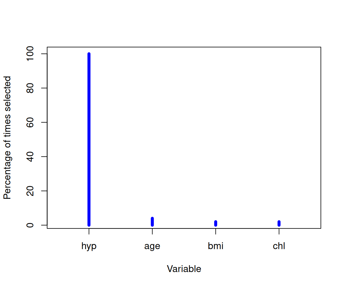
Selection frequency of the variables for the optimal number of clusters:
y <- getvariablesfrequency(minhanes1clust)
y
#> $percfreq
#> [1] 100   4   2   2
#>
#> $varnames
#> [1] "hyp" "age" "bmi" "chl"
plot(y$percfreq, type = "h", main = "", xlab = "Variable", ylab = "Percentage of times selected",
     xlim = 0.5 + c(0, length(y$varnames)), lwd = 5, col = "blue", xaxt = "n")
axis(1, at = 1:length(y$varnames), labels = y$varnames)
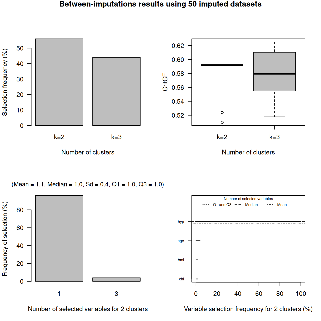
Graphical representation of the results:
plot(minhanes1clust)
Summary for the optimal number of clusters:
summary(minhanes1clust)
#> Warning in summary.miclust(minhanes1clust): 'quantilevars' not provided. Setting it to 0.5.
#>
#> Results using:
#>     50 imputed datasets for the cluster analysis
#>     100 imputed datasets for the descriptive summary
#>     2 as the final number of clusters
#> -----------------------------------------------------------
#>
#> Presence of the variables in the subset of selected variables:
#>   Variable Presence(%)
#> 1      hyp         100
#> 2      age           4
#> 3      bmi           2
#> 4      chl           2
#>
#> Selected variables:
#> [1] "hyp"
#>
#> Cohen's kappa between-imputations distribution (99 comparisons):
#>  2.5%   25%   50%  mean   75% 97.5%
#>  0.48  0.65  0.78  0.75  0.88  1.00
#>
#> Between-imputation clusters size distribution (100 imputations):
#>           size min. 2.5% 25% 50% mean 75% 97.5% max.
#> cluster 1    7    4    4   6   7  6.5   7     9   10
#> cluster 2   18   15   16  18  18 18.5  19    21   21
#>
#> Probability of assignment to the cluster distribution (100 imputations):
#>                        min   Q1 Q2 Q3 max
#> Assigned to cluster 1 0.51 0.54  1  1   1
#> Assigned to cluster 2 0.52 0.93  1  1   1
#>
#> Within-cluster summary (100 imputations) [%miss.;mean;sd]:
#>     %miss.            cl.1            cl.2
#> hyp     32 42.86;2.00;0.00 27.78;1.00;0.00
References
The methodology used in the package is described in
- Basagaña X, Barrera-Gómez J, Benet M, Antó JM, Garcia-Aymerich J. A Framework for Multiple Imputation in Cluster Analysis. American Journal of Epidemiology. 2013;177(7):718-725. https://doi.org/10.1093/aje/kws289