mcstatsim
Monte Carlo Statistical Simulation Tools Using a Functional Approach
A lightweight toolkit for Monte Carlo simulation studies built around a higher-order, functional-style interface: the simulation is expressed as a function of its parameters and mapped over a grid of conditions by a single driver function, which handles iteration, parallelism, reproducible per-replication random-number streams, error capture and result assembly. Also provides ready-to-use performance measures with Monte Carlo standard errors, a summary layer, and diagnostic plots.
mcstatsim


About
mcstatsim is a lightweight, functional-style toolkit for Monte Carlo
simulation studies. Its core is a higher-order driver, runsim(): you write
the simulation as a function of its parameters, and runsim() maps it over a
grid of conditions, owning the iteration, parallelism, reproducible
random-number streams, error capture and result assembly. Around it the package
ships ready-to-use performance measures, an evaluation layer that turns
raw replicates into a tidy results table, and diagnostic plots.
The only hard dependency is functionals. ggplot2 is used by the plotting
helpers and is optional.
How it works
runsim() takes a grid of conditions (one row per scenario), a simulation
function whose arguments match the grid columns, and the number of
replications. It builds one flat list of n * nrow(grid) jobs, runs them in a
single load-balanced parallel pass, and row-binds the results into a data frame
with the grid columns, the quantities returned by the simulation function, and a
replication index ID.
Installation
install.packages("mcstatsim")                    # released version
# install.packages("remotes")
remotes::install_github("ielbadisy/mcstatsim")   # development version
A complete example
We evaluate the normal-theory 95% confidence interval for a mean when the data
are drawn either from a normal distribution or from a skewed (centred
log-normal) distribution, across three sample sizes. The true mean is 0 in
every cell, so we expect bias near zero and coverage near 0.95, but the
t-interval is known to under-cover under skew at small n.
1. Simulation function and grid
library(mcstatsim)

sim_mean_ci <- function(n, dist) {
  x <- if (dist == "normal") rnorm(n) else rlnorm(n) - exp(0.5)  # both have mean 0
  est <- mean(x)
  se  <- sd(x) / sqrt(n)
  crit <- qt(0.975, df = n - 1)
  data.frame(
    est      = est,
    lo       = est - crit * se,
    hi       = est + crit * se,
    true_val = 0
  )
}

grid <- expand.grid(n = c(10, 30, 100), dist = c("normal", "lognormal"),
                    stringsAsFactors = FALSE)
grid
#>     n      dist
#> 1  10    normal
#> 2  30    normal
#> 3 100    normal
#> 4  10 lognormal
#> 5  30 lognormal
#> 6 100 lognormal
2. Run the simulation
seed gives every job its own independent L'Ecuyer-CMRG stream, so the run is
reproducible and does not depend on the number of cores.
res <- runsim(
  n           = 2000,
  grid_params = grid,
  sim_func    = sim_mean_ci,
  seed        = 2025,
  num_cores   = 2,
  show_progress = FALSE
)

head(res)
#>     n      dist          est          lo         hi true_val ID
#> 1  10    normal  0.433489939 -0.35003582 1.21701569        0  1
#> 2  30    normal -0.363420104 -0.74905905 0.02221884        0  1
#> 3 100    normal  0.162087539 -0.03781371 0.36198879        0  1
#> 4  10 lognormal  0.292061905 -1.37614955 1.96027336        0  1
#> 5  30 lognormal -0.147570162 -0.56076715 0.26562683        0  1
#> 6 100 lognormal  0.004260512 -0.37423359 0.38275461        0  1
nrow(res)
#> [1] 12000
3. Turn replicates into a performance table
perf <- summarise_sim(
  res,
  by = c("n", "dist"),
  measures = list(
    bias     = ~ calc_bias(est, true_val[1]),
    coverage = ~ calc_coverage(lo, hi, true_val[1]),
    width    = ~ calc_width(lo, hi)
  )
)
perf
#>     n      dist n_sim    bias bias_mcse coverage coverage_mcse  width
#> 1  10 lognormal  2000 -0.0113    0.0153   0.8370        0.0083 2.4341
#> 2  10    normal  2000  0.0092    0.0068   0.9515        0.0048 1.3913
#> 3  30 lognormal  2000 -0.0009    0.0090   0.8750        0.0074 1.4440
#> 4  30    normal  2000  0.0016    0.0042   0.9455        0.0051 0.7402
#> 5 100 lognormal  2000 -0.0007    0.0048   0.9190        0.0061 0.8079
#> 6 100    normal  2000 -0.0004    0.0023   0.9470        0.0050 0.3957
#>   width_mcse
#> 1     0.0396
#> 2     0.0075
#> 3     0.0181
#> 4     0.0022
#> 5     0.0062
#> 6     0.0006
Each calc_* measure contributes its estimate and its Monte Carlo standard
error (the *_mcse columns). Numeric columns are rounded to digits (default
4); pass digits = NULL to summarise_sim() for full precision.
4. Diagnostics
Check that no replicate produced a non-finite estimate:
check_estimates(res, by = c("n", "dist"))
#> [1] n        dist     column   n_bad    n_total  prop_bad
#> <0 rows> (or 0-length row.names)
How many replications would we need to pin the coverage MCSE down to 0.0025?
data.frame(perf[c("n", "dist")],
           coverage_mcse = round(perf$coverage_mcse, 4),
           reps_for_0.0025 = mcse_target(perf$coverage_mcse, perf$n_sim, target = 0.0025))
#>     n      dist coverage_mcse reps_for_0.0025
#> 1  10 lognormal        0.0083           22045
#> 2  10    normal        0.0048            7373
#> 3  30 lognormal        0.0074           17524
#> 4  30    normal        0.0051            8324
#> 5 100 lognormal        0.0061           11908
#> 6 100    normal        0.0050            8000
5. Plots
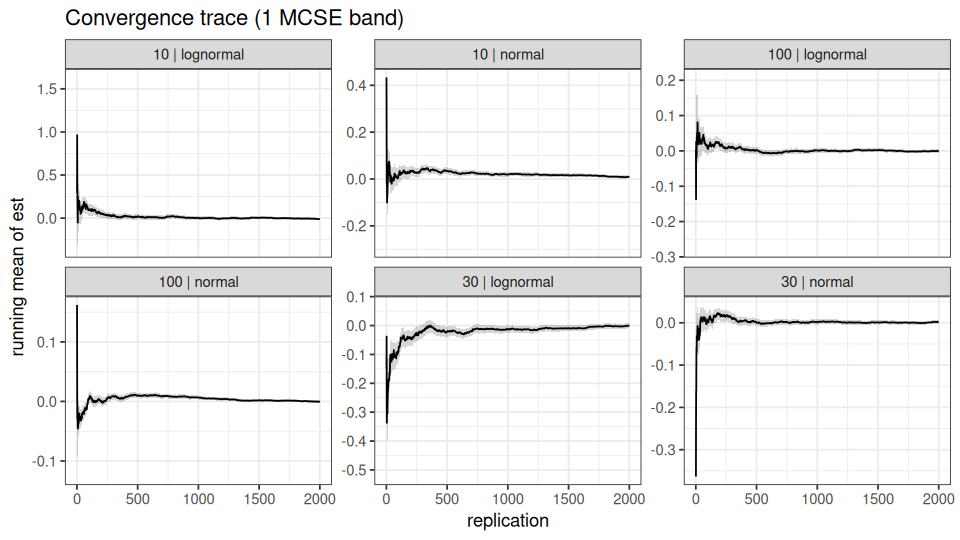
Convergence trace. The running mean of the point estimate with a Monte Carlo standard-error band, one panel per condition:
plot_convergence(res, "est", by = c("n", "dist"))
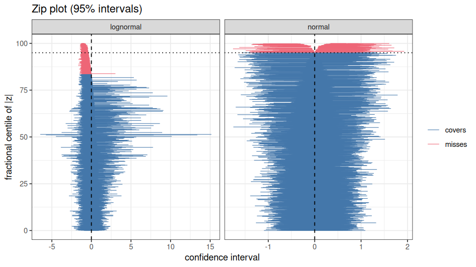
Zip plot (Morris, White and Crowther, 2019). Confidence intervals sorted by
the extremeness of their z-statistic and coloured by whether they cover; a
well-calibrated interval fills the panel up to the nominal line in the
“covers” colour. Shown here for n = 10:
plot_zip(res[res$n == 10, ], "lo", "hi", "true_val", by = "dist")
Performance across the design. Coverage with a +/- 2 MCSE bar against
the nominal 0.95 line:
plot_performance(perf, "coverage", x = "n", colour = "dist", ref = 0.95)
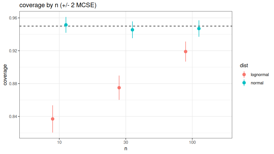
The log-normal intervals under-cover at n = 10 (the zip plot shows the misses
concentrated on one side, the signature of skew) and climb back toward 0.95 as
n grows. The normal-data intervals sit on 0.95 throughout.
Reproducibility and error handling
a <- runsim(200, grid, sim_mean_ci, seed = 1, num_cores = 1, show_progress = FALSE)
b <- runsim(200, grid, sim_mean_ci, seed = 1, num_cores = 4, show_progress = FALSE)
identical(a$est, b$est)
#> [1] TRUE
If a simulation function errors on some cells, on_error = "warn" (or
"omit") drops those jobs and records them in attr(x, "errors"), which
failure_summary() aggregates per condition. Warnings raised inside the
simulation function are kept in attr(x, "warnings").
fragile <- function(n, dist) {
  if (dist == "lognormal" && n == 10 && runif(1) < 0.1) stop("fit did not converge")
  sim_mean_ci(n, dist)
}
r <- runsim(200, grid, fragile, seed = 1, on_error = "omit",
            num_cores = 1, show_progress = FALSE)
nrow(r)
#> [1] 1179
failure_summary(r)
#>    n      dist n_failed failure_rate        example_error
#> 1 10 lognormal       21        0.105 fit did not converge
A save_path makes a long run resumable: the result is checkpointed after
each chunk of checkpoint_every replications, and re-running runsim() with
the same save_path, n, grid_params and seed loads the completed
replications and runs only the rest. A resumed run reproduces an uninterrupted
one exactly.
ckpt <- tempfile(fileext = ".rds")
r1 <- runsim(200, grid, sim_mean_ci, seed = 1, save_path = ckpt,
             checkpoint_every = 50, num_cores = 1, show_progress = FALSE)
identical(r1$est, a$est)
#> [1] TRUE
Performance measures
calc_bias(), calc_variance(), calc_mse(), calc_rmse(),
calc_coverage(), calc_width(), calc_rejection_rate(),
calc_relative_bias(), calc_relative_mse(), calc_relative_rmse(). Each
returns the estimate together with its Monte Carlo standard error, rounded to
digits (default 4; NULL for full precision). They can be used on their own
or inside summarise_sim().
est <- res$est[res$n == 30 & res$dist == "normal"]
calc_bias(est, 0)
#> $bias
#> [1] 0.0016
#>
#> $bias_mcse
#> [1] 0.0042
calc_rmse(est, 0, digits = NULL)
#> $rmse
#> [1] 0.1860117
#>
#> $rmse_mcse
#> [1] 0.003563415
Lower-level helpers
mcpmap() maps a function over equal-length named lists in parallel (via
functionals), and combine_df() row-binds a list of lists of data frames,
adding a source ID. runsim() covers most use cases; these are there for
custom drivers.
mcpmap(list(a = 1:3, b = 4:6), function(a, b) a + b, num_cores = 1,
       show_progress = FALSE)
#> [[1]]
#> [1] 5
#>
#> [[2]]
#> [1] 7
#>
#> [[3]]
#> [1] 9
Features
- Higher-order, declarative interface: write the simulation as a function;
runsim()maps it over the design. - Reproducible parallelism: per-job RNG streams; results independent of core count.
- Robustness: per-cell error/warning capture, checkpoint/resume for long runs.
- Evaluation layer:
summarise_sim()plus a full set of MCSE-aware measures. - Diagnostics: convergence traces, zip plots, performance plots, non-finite checks.
Learn more
The package vignette, “Monte Carlo simulation studies with mcstatsim” (PDF),
walks through runsim(), reproducible RNG, error handling, checkpoint/resume,
summarise_sim(), the calc_* measures, diagnostics and plots, with a worked
case study:
vignette("mcstatsim", package = "mcstatsim")
Citation
To cite mcstatsim in publications, use:
citation("mcstatsim")
#> To cite mcstatsim in publications, use:
#>
#>   El Badisy I (2026). _mcstatsim: Monte Carlo Statistical Simulation
#>   Tools Using a Functional Approach_. R package version 0.9.2,
#>   <https://CRAN.R-project.org/package=mcstatsim>.
#>
#> A BibTeX entry for LaTeX users is
#>
#>   @Manual{,
#>     title = {mcstatsim: Monte Carlo Statistical Simulation Tools Using a Functional Approach},
#>     author = {Imad {El Badisy}},
#>     year = {2026},
#>     note = {R package version 0.9.2},
#>     url = {https://CRAN.R-project.org/package=mcstatsim},
#>   }
Contributing
Contributions are welcome. Please feel free to open an issue or submit a pull request.