lspline
Linear Splines with Convenient Parametrisations
Linear splines with convenient parametrisations such that (1) coefficients are slopes of consecutive segments or (2) coefficients are slope changes at consecutive knots. Knots can be set manually or at break points of equal-frequency or equal-width intervals covering the range of 'x'. The implementation follows Greene (2003), chapter 7.2.5.
lspline: Linear Splines with Convenient Parametrisations

Linear splines with convenient parametrisations such that
- coefficients are slopes of consecutive segments
- coefficients capture slope change at consecutive knots
Knot locations can be specified
- manually (
lspline()) - at breaks dividing the range of
xintoqequal-frequency intervals (qlspline()) - at breaks dividing the range of
xintonequal-width intervals (elspline())
Examples
Examples of using lspline(), qlspline(), and elspline(). We will use the following artificial data with knots at x=5 and x=10
set.seed(666)
n <- 200
d <- data.frame(
  x = scales::rescale(rchisq(n, 6), c(0, 20))
)
d$interval <- findInterval(d$x, c(5, 10), rightmost.closed = TRUE) + 1
d$slope <- c(2, -3, 0)[d$interval]
d$intercept <- c(0, 25, -5)[d$interval]
d$y <- with(d, intercept + slope * x + rnorm(n, 0, 1))
Plotting y against x:
library(ggplot2)
fig <- ggplot(d, aes(x=x, y=y)) +
  geom_point(aes(shape=as.character(slope))) +
  scale_shape_discrete(name="Slope") +
  theme_bw()
fig
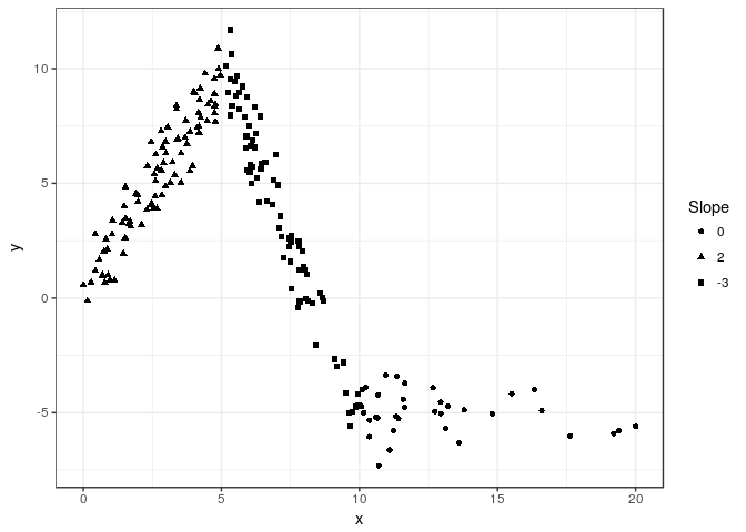
The slopes of the consecutive segments are 2, -3, and 0.
Setting knot locations manually
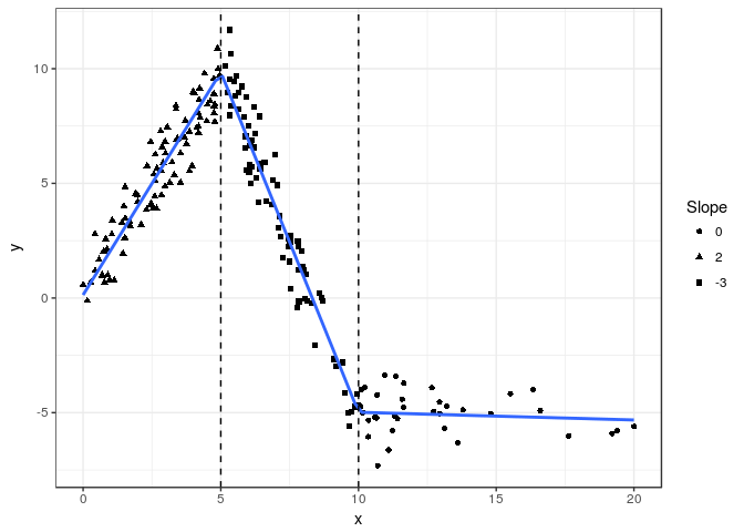
We can parametrize the spline with slopes of individual segments (default marginal=FALSE):
library(lspline)
m1 <- lm(y ~ lspline(x, c(5, 10)), data=d)
knitr::kable(broom::tidy(m1))
| term | estimate | std.error | statistic | p.value |
|---|---|---|---|---|
| (Intercept) | 0.1343204 | 0.2148116 | 0.6252941 | 0.5325054 |
| lspline(x, c(5, 10))1 | 1.9435458 | 0.0597698 | 32.5171747 | 0.0000000 |
| lspline(x, c(5, 10))2 | -2.9666750 | 0.0503967 | -58.8664832 | 0.0000000 |
| lspline(x, c(5, 10))3 | -0.0335289 | 0.0518601 | -0.6465255 | 0.5186955 |
Or parametrize with coeficients measuring change in slope (with marginal=TRUE):
m2 <- lm(y ~ lspline(x, c(5,10), marginal=TRUE), data=d)
knitr::kable(broom::tidy(m2))
| term | estimate | std.error | statistic | p.value |
|---|---|---|---|---|
| (Intercept) | 0.1343204 | 0.2148116 | 0.6252941 | 0.5325054 |
| lspline(x, c(5, 10), marginal = TRUE)1 | 1.9435458 | 0.0597698 | 32.5171747 | 0.0000000 |
| lspline(x, c(5, 10), marginal = TRUE)2 | -4.9102208 | 0.0975908 | -50.3143597 | 0.0000000 |
| lspline(x, c(5, 10), marginal = TRUE)3 | 2.9331462 | 0.0885445 | 33.1262479 | 0.0000000 |
The coefficients are
lspline(x, c(5, 10), marginal = TRUE)1- the slope of the first segmentlspline(x, c(5, 10), marginal = TRUE)2- the change in slope at knot x = 5; it is changing from 2 to -3, so by -5lspline(x, c(5, 10), marginal = TRUE)3- tha change in slope at knot x = 10; it is changing from -3 to 0, so by 3
The two parametrisations (obviously) give identical predicted values:
all.equal( fitted(m1), fitted(m2) )
## [1] TRUE
graphically
fig +
  geom_smooth(method="lm", formula=formula(m1), se=FALSE) +
  geom_vline(xintercept = c(5, 10), linetype=2)
Knots at n equal-length intervals
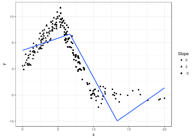
Function elspline() sets the knots at points dividing the range of x into n equal length intervals.
m3 <- lm(y ~ elspline(x, 3), data=d)
knitr::kable(broom::tidy(m3))
| term | estimate | std.error | statistic | p.value |
|---|---|---|---|---|
| (Intercept) | 3.5484817 | 0.4603827 | 7.707678 | 0.00e+00 |
| elspline(x, 3)1 | 0.4652507 | 0.1010200 | 4.605529 | 7.40e-06 |
| elspline(x, 3)2 | -2.4908385 | 0.1167867 | -21.328105 | 0.00e+00 |
| elspline(x, 3)3 | 0.9475630 | 0.2328691 | 4.069080 | 6.84e-05 |
Graphically
fig +
  geom_smooth(aes(group=1), method="lm", formula=formula(m3), se=FALSE, n=200)
Knots at quantiles of x
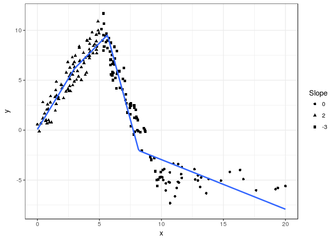
Function qlspline() sets the knots at points dividing the range of x into q equal-frequency intervals.
m4 <- lm(y ~ qlspline(x, 4), data=d)
knitr::kable(broom::tidy(m4))
| term | estimate | std.error | statistic | p.value |
|---|---|---|---|---|
| (Intercept) | 0.0782285 | 0.3948061 | 0.198144 | 0.8431388 |
| qlspline(x, 4)1 | 2.0398804 | 0.1802724 | 11.315548 | 0.0000000 |
| qlspline(x, 4)2 | 1.2675186 | 0.1471270 | 8.615132 | 0.0000000 |
| qlspline(x, 4)3 | -4.5846478 | 0.1476810 | -31.044273 | 0.0000000 |
| qlspline(x, 4)4 | -0.4965858 | 0.0572115 | -8.679818 | 0.0000000 |
Graphically
fig +
  geom_smooth(method="lm", formula=formula(m4), se=FALSE, n=200)
Installation
Stable version from CRAN or development version from GitHub with
devtools::install_github("mbojan/lspline", build_vignettes=TRUE)
Acknowledgements
Inspired by Stata command mkspline and function ares::lspline from Junger & Ponce de Leon (2011). As such, the implementation follows Greene (2003), chapter 7.5.2.
- Greene, William H. (2003) Econometric analysis. Pearson Education
- Junger & Ponce de Leon (2011)
ares: Environment air pollution epidemiology: a library for timeseries analysis. R package version 0.7.2 retrieved from CRAN archives.