Linear Specification Testing

Tests whether the linear hypothesis of a model is correct specified using Dominguez-Lobato test. Also Ramsey's RESET (Regression Equation Specification Error Test) test is implemented and Wald tests can be carried out. Although RESET test is widely used to test the linear hypothesis of a model, Dominguez and Lobato (2019) proposed a novel approach that generalizes well known specification tests such as Ramsey's. This test relies on wild-bootstrap; this package implements this approach to be usable with any function that fits linear models and is compatible with the update() function such as 'stats'::lm(), 'lfe'::felm() and 'forecast'::Arima(), for ARMA (autoregressive–moving-average) models. Also the package can handle custom statistics such as Cramer von Mises and Kolmogorov Smirnov, described by the authors, and custom distributions such as Mammen (discrete and continuous) and Rademacher. Manuel A. Dominguez & Ignacio N. Lobato (2019) .

lineartestr

The goal of lineartestr is to contrast the linear hypothesis of a model:

Using the Domínguez-Lobato test which relies on wild-bootstrap. Also the Ramsey RESET test is implemented.

Installation

You can install the released version of lineartestr from CRAN with:

install.packages("lineartestr")

And the development version from GitHub with:

# install.packages("devtools")
devtools::install_github("FedericoGarza/lineartestr")

References

• Manuel A. Domínguez and Ignacio N. Lobato (2019). Specification testing with estimated variables. Econometric Reviews.

Cite as

• Garza F (2020). lineartestr: Test the linear specification of a model. R package version 1.0.0, https://github.com/FedericoGarza/lineartestr.

Examples

Simplest linear models using lm function

library(lineartestr)

x <- 1:100
y <- 1:100

lm_model <- lm(y~x)

dl_test <- dominguez_lobato_test(lm_model)

dplyr::glimpse(dl_test$test)
#> Observations: 1
#> Variables: 7
#> $ name_distribution <chr> "rnorm"
#> $ name_statistic    <chr> "cvm_value"
#> $ statistic         <dbl> 7.562182e-29
#> $ p_value           <dbl> 0.4066667
#> $ quantile_90       <dbl> 2.549223e-28
#> $ quantile_95       <dbl> 3.887169e-28
#> $ quantile_99       <dbl> 6.359681e-28

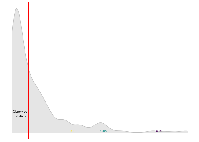
Also lineartestr can plot the results

plot_dl_test(dl_test)

Run in parallel!

library(lineartestr)
x_p <- 1:1e5
y_p <- 1:1e5

lm_model_p <- lm(y_p~x_p)

dl_test_p <- dominguez_lobato_test(lm_model_p, n_cores=7)

dplyr::glimpse(dl_test_p$test)
#> Observations: 1
#> Variables: 7
#> $ name_distribution <chr> "rnorm"
#> $ name_statistic    <chr> "cvm_value"
#> $ statistic         <dbl> 6.324343e-21
#> $ p_value           <dbl> 0.3566667
#> $ quantile_90       <dbl> 1.902697e-20
#> $ quantile_95       <dbl> 2.532663e-20
#> $ quantile_99       <dbl> 4.141126e-20

RESET test can also be used to test the linear hypothesis

library(lineartestr)

x <- 1:100 + rnorm(100)
y <- 1:100

lm_model <- lm(y~x)

r_test <- reset_test(lm_model)

dplyr::glimpse(r_test)
#> Observations: 1
#> Variables: 6
#> $ statistic   <dbl> 0.7797557
#> $ p_value     <dbl> 0.6771396
#> $ df          <int> 2
#> $ quantile_90 <dbl> 4.60517
#> $ quantile_95 <dbl> 5.991465
#> $ quantile_99 <dbl> 9.21034

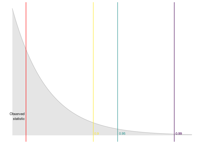
An then we can plot the results

plot_reset_test(r_test)

Linear fixed effects with lfe

library(lineartestr)
library(dplyr)
#> 
#> Attaching package: 'dplyr'
#> The following objects are masked from 'package:stats':
#> 
#>     filter, lag
#> The following objects are masked from 'package:base':
#> 
#>     intersect, setdiff, setequal, union
library(lfe)
#> Loading required package: Matrix

# This example was taken from https://www.rdocumentation.org/packages/lfe/versions/2.8-5/topics/felm
x <- rnorm(1000)
x2 <- rnorm(length(x))
# Individuals and firms
id <- factor(sample(20,length(x),replace=TRUE))
firm <- factor(sample(13,length(x),replace=TRUE))
# Effects for them
id.eff <- rnorm(nlevels(id))
firm.eff <- rnorm(nlevels(firm))
# Left hand side
u <- rnorm(length(x))
y <- x + 0.5*x2 + id.eff[id] + firm.eff[firm] + u
new_y <- y + rnorm(length(y))
## Estimate the model
est <- lfe::felm(y ~ x + x2 | id + firm)


## Testing the linear hypothesis and plotting results
dominguez_lobato_test(est, n_cores = 7) %>%
  plot_dl_test()

ARMA models

library(lineartestr)
library(dplyr)

x <- rnorm(100)**3

arma_model <- forecast::Arima(x, order = c(1, 0, 1))
#> Registered S3 method overwritten by 'xts':
#>   method     from
#>   as.zoo.xts zoo
#> Registered S3 method overwritten by 'quantmod':
#>   method            from
#>   as.zoo.data.frame zoo
#> Registered S3 methods overwritten by 'forecast':
#>   method             from    
#>   fitted.fracdiff    fracdiff
#>   residuals.fracdiff fracdiff

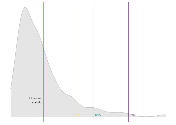
dominguez_lobato_test(arma_model) %>%
  plot_dl_test()