Compare Big Datasets to the Uniform Distribution

A quantile-quantile plot can be used to compare a sample of p-values to the uniform distribution. But when the dataset is big (i.e. > 1e4 p-values), plotting the quantile-quantile plot can be slow. geom_QQ uses all the data to calculate the quantiles, but thins it out in a way that focuses on points near zero before plotting to speed up plotting and decrease file size, when vector graphics are stored.

gg_QQ_unif

ggbigQQ extends ggplot2 to allow the user to make a quantile-quantile plot with a big dataset. Specifically, geom_big_qq uses all the data provided to calculate quantiles, but drops points that would overplot before plotting. <!-- There's no use in having ten thousand points in a plot to define a line -- we can't even see most of them! --> In this way, the resultant figure maintains all the accuracy of a Q-Q plot made with a large dataset, but renders as fast as one from a smaller dataset and, when stored as a vector graphic, has the file size of a Q-Q plot from a smaller dataset.

Examples

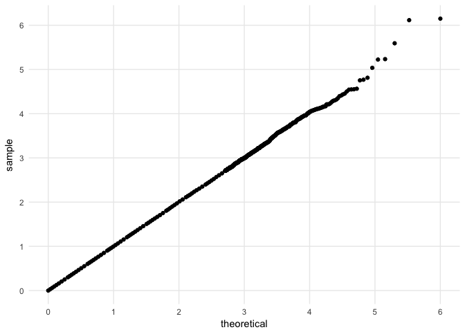
Here's an example where geom_qq takes 14 seconds to render the plot on my intel i5 and geom_big_qq takes 1 second to produce the same plot.

set.seed(27599)
d <- data.frame(s = runif(n = 5e5))

# # takes 14 seconds
# d %>%
#   ggplot(mapping = aes(sample = s)) +
#   geom_qq(distribution = qunif) +
#   QQ_scale_x() +
#   QQ_scale_y()


# takes 1 second
d %>%
  ggplot(mapping = aes(sample = s)) +
  geom_QQ_unif() +
  scale_x_QQ() +
  scale_y_QQ() +
  theme_minimal()

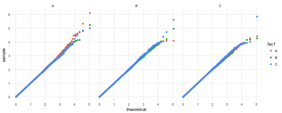
This geom works with other aesthetics, too.

set.seed(27599)
n <- 5e5
d <- data.frame(fac1 = sample(x = LETTERS[1:3], size = n, replace = TRUE),
                fac2 = sample(x = LETTERS[1:3], size = n, replace = TRUE),
                s = runif(n = n))

# takes 1 second
d %>%
  ggplot(mapping = aes(sample = s, color = fac1)) +
  geom_QQ_unif() +
  facet_wrap(~ fac2) +
  scale_x_QQ() +
  scale_y_QQ() +
  theme_minimal()