Estimate Graph Dimension using Cross-Validated Eigenvalues

Cross-validated eigenvalues are estimated by splitting a graph into two parts, the training and the test graph. The training graph is used to estimate eigenvectors, and the test graph is used to evaluate the correlation between the training eigenvectors and the eigenvectors of the test graph. The correlations follow a simple central limit theorem that can be used to estimate graph dimension via hypothesis testing, see Chen et al. (2021) for details.

gdim

gdim estimates graph dimension using cross-validated eigenvalues, via the graph-splitting technique developed in https://arxiv.org/abs/2108.03336. Theoretically, the method works by computing a special type of cross-validated eigenvalue which follows a simple central limit theorem. This allows users to perform hypothesis tests on the rank of the graph.

Installation

You can install gdim from CRAN with:

install.packages("gdim")

# to get the development version from GitHub:
install.packages("pak")
pak::pak("RoheLab/gdim")

Example

eigcv() is the main function in gdim. The single required parameter for the function is the maximum possible dimension, k_max.

In the following example, we generate a random graph from the stochastic block model (SBM) with 1000 nodes and 5 blocks (as such, we would expect the estimated graph dimension to be 5).

library(fastRG)
#> Loading required package: Matrix

B <- matrix(0.1, 5, 5)
diag(B) <- 0.3

model <- sbm(
  n = 1000,
  B = B,
  expected_degree = 40,
  poisson_edges = FALSE,
  allow_self_loops = FALSE
)

A <- sample_sparse(model)

Here, A is the adjacency matrix.

Now, we call the eigcv() function with k_max=10 to estimate graph dimension.

library(gdim)

eigcv_result <- eigcv(A, k_max = 10)
#> 'as(<dsCMatrix>, "dgCMatrix")' is deprecated.
#> Use 'as(., "generalMatrix")' instead.
#> See help("Deprecated") and help("Matrix-deprecated").
eigcv_result
#> Estimated graph dimension:    5
#> 
#> Number of bootstraps:         10
#> Edge splitting probabaility:  0.1
#> Significance level:       0.05
#> 
#>  ------------ Summary of Tests ------------
#>   k          z        pvals         padj
#>   1 41.1972023 0.000000e+00 0.000000e+00
#>   2  6.5483842 2.908147e-11 2.908147e-11
#>   3  6.2885741 1.601976e-10 1.601976e-10
#>   4  6.9601015 1.700138e-12 1.700138e-12
#>   5  7.1673010 3.824537e-13 3.824537e-13
#>   6 -0.3594110 6.403562e-01 6.403562e-01
#>   7 -0.2062852 5.817159e-01 5.817159e-01
#>   8 -0.6096004 7.289367e-01 7.289367e-01
#>   9 -0.7202233 7.643062e-01 7.643062e-01
#>  10 -0.6707828 7.488205e-01 7.488205e-01

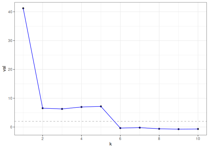
In this example, eigcv() suggests k=5.

To visualize the result, use plot() which returns a ggplot object. The function displays the test statistic (z score) for each hypothesized graph dimension.

plot(eigcv_result)

Reference

Chen, Fan, Sebastien Roch, Karl Rohe, and Shuqi Yu. “Estimating Graph Dimension with Cross-Validated Eigenvalues.” ArXiv:2108.03336 [Cs, Math, Stat], August 6, 2021. https://arxiv.org/abs/2108.03336.