Cumulative Calibration Assessment for Prediction Models

Tools for visualization of, and inference on, the calibration of prediction models on the cumulative domain. This provides a method for evaluating calibration of risk prediction models without having to group the data or use tuning parameters (e.g., loess bandwidth). This package implements the methodology described in Sadatsafavi and Petkau (2024) . The core of the package is cumulcalib(), which takes in vectors of binary responses and predicted risks. The package also implements non-parametric assessment of the calibration of individualized treatment effect (ITE) models using data from a randomized trial, via cumulcalibITE(), as described in Sadatsafavi et al. (2026) . The plot() and summary() methods are implemented for the results returned by cumulcalib() and cumulcalibITE().

cumulcalib

cumulcalib provides non-parametric, tuning-parameter-free assessment of model calibration on the cumulative-sum domain, for two settings:

Risk prediction models — cumulcalib() assesses the calibration of predicted risks (Sadatsafavi and Petkau 2024, https://doi.org/10.1002/sim.10138).
Individualized treatment effect (ITE) models — cumulcalibITE() assesses the moderate calibration of predicted treatment benefits using data from a randomized trial (Sadatsafavi et al. 2026, https://doi.org/10.1002/sim.70724).

The package comes with two tutorials (vignettes), which you can view after installing the package:

vignette("tutorial", package = "cumulcalib")     # risk prediction models
vignette("tutorialITE", package = "cumulcalib")  # ITE models

Installation

The package can be installed from CRAN:

install.packages("cumulcalib")

You can also install the development version, which includes the individualized treatment effect (ITE) functionality, from GitHub with:

# install.packages("remotes") #this package is necessary to connect to github
remotes::install_github("resplab/cumulcalib")

Example

library(cumulcalib)

set.seed(1)
p <- rbeta(1000, 1,5)
y <- rbinom(1000,1,p)

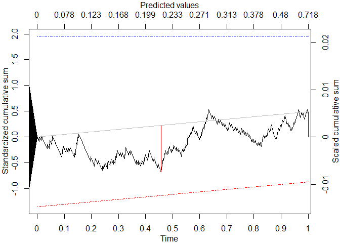
res <- cumulcalib(y, p)

summary(res)
#> Moderate calibration assessment of predicted risks
#> C_n (mean calibration error): 0.00532270104567871
#> C* (maximum cumulative calibration error): 0.00740996981029672  (observed risk < predicted)
#>   Location of maximum cumulative error: time = 0.457280572542993, predicted risk = 0.217915058214255
#> Method: Two-part Brownian bridge (BB)
#> S_n (Z score for mean calibration error): 0.489295496431201
#> B* (test statistic for maximum absolute bridged calibration error): 0.904915434767163
#> Component-wise p-values: mean calibration=0.624632509005787 | Distance (bridged)=0.385979705481866
#> Combined p-value (Fisher's method): 0.584068794836004
plot(res)