Difference-in-Differences with a Continuous Treatment

Provides methods for difference-in-differences with a continuous treatment and staggered treatment adoption. Includes estimation of treatment effects and causal responses as a function of the dose, event studies indexed by length of exposure to the treatment, and aggregation into overall average effects. Uniform inference procedures are included, along with both parametric and nonparametric models for treatment effects. The methods are based on Callaway, Goodman-Bacon, and Sant'Anna (2025) .

contdid

An R package for difference-in-differences with a continuous treatment.

Installation

You can install the development version of contdid from GitHub with:

# install.packages("devtools")
devtools::install_github("bcallaway11/contdid")

library(contdid)

Package Status: Alpha Version

This is an alpha version of the contdid package. The core features are implemented and functional, but the package remains under active development. The API may change, and additional functionality is planned.

We welcome feedback and encourage users to report bugs or other issues via the GitHub Issues page.

✅ Currently Supported

• ☑️ Continuous treatments
• ☑️ Staggered treatment adoption (i.e., more than two periods and variation in timing across units)
• ☑️ Aggregations into dose-specific ATT’s or ACRT’s
• ☑️ Aggregations into ATT or ACRT versions of event studies
• ☑️ User-specified flexible parametric models for treatment effects as a function of the dose

🚫 Not Yet Supported

• ❌ Discrete treatments

  • This is straightforward and could be implemented by users directly, but we don’t have it in the package yet.

• ⚠️ Data-driven models for treatment effects as a function of the dose

  • We have this working for cases without staggered adoption, but it is not yet implemented for staggered adoption. We plan to add this in the future.

• ❌ Repeated cross-sections data

• ❌ Unbalanced panel data

• ❌ Doses that vary over time

  • Not sure if we will ever support this, or maybe only in limited contexts._

• ❌ Including covariates

Conceptual Setup

Below, we give several examples of how to estimate causal effect parameters using the contdid package.

At a high level, the interface is basically the same as for the did package and for packages that rely on the ptetools backend, with only a few pieces of additional information being required. First, the name of the continuous treatment variable should be passed through the dname argument.

The cont_did function expects the continuous treatment variable to behave in certain ways:

1. It needs to be time-invariant.

2. It should be set to its time-invariant value in pre-treatment periods. This is just a convention of the package, but, in particular, you should not have the treatment variable coded as being 0 in pre-treatment periods.

3. For units that don’t participate in the treatment in any time period, the treatment variable just needs to be time-invariant. In some applications, e.g., the continuous treatment variable may be defined for units that don’t actually participate in the treatment. In other applications, it may not be defined for units that do not participate in the treatment. The function behaves the same way in either case.

Next, the other important parameters are target_parameter, aggregation, and treatment_type:

• target_parameter can either be “level” or “slope”. If “level”, then the function will calculate ATT parameters. If set to be “slope”, then the function will calculate ACRT parameters—these are causal response parameters that are derivatives of the ATT parameters. Our paper Callaway, Goodman-Bacon, and Sant’Anna (2024) points out some complications for interpreting these derivative type parameters under the most commonly invoked version of the parallel trends assumption.

• aggregation can either by “eventstudy” or “dose”. For “eventstudy”, depending on the value of the target_parameter argument, the function will provide either the average ATT across different event times or the average ACRT across different event times. For “dose”, the function will average across all time periods and report average affects across different values of the continuous treatment. For the “dose” aggregation, results are calculated for both ATT and ACRT and can be displayed by providing different arguments to plotting functions (see example below).

• treatment_type can either be “continuous” or “discrete”. Currently only “continuous” is supported. In this case, the code proceeds as if the treatment really is continuous. The estimate are computed nonparametrically using B-splines. The user can control the number of knots and the degree of the B-splines using the num_knots and degree arguments. The defaults are num_knots=0 and degree=1 which amounts to estimating ATT(d) by estimating a linear model in the continuous treatment among treated units and subtracting the average outcome among the comparison units.

Examples

With a continuous treatment, the underlying building blocks are treatment effects that are local to a particular timing group g in a particular time period t that experienced a particular value of the treatment d. These treatment affects are relatively high-dimensional, and most applications are likely to involve aggregating/combining these underlying parameters. We focus on aggregations that (i) average across timing-groups and time periods to given average treatment effect parameters as a function of the dose d or (ii) averages across doses and partially across timing group and time periods in order to give event studies.

For the results below, we will simulate some data, where the continuous treatment D has no effect on the outcome.

# Simulate data
set.seed(1234)
df <- simulate_contdid_data(
  n = 5000,
  num_time_periods = 4,
  num_groups = 4,
  dose_linear_effect = 0,
  dose_quadratic_effect = 0
)
head(df)
#>   id G          D time_period         Y
#> 1  1 2 0.08593221           1 0.3579583
#> 2  1 2 0.08593221           2 5.2354694
#> 3  1 2 0.08593221           3 3.2717079
#> 4  1 2 0.08593221           4 4.3988042
#> 5  2 4 0.17217781           1 5.9743351
#> 6  2 4 0.17217781           2 5.8463051

Case 1: Dose Aggregation

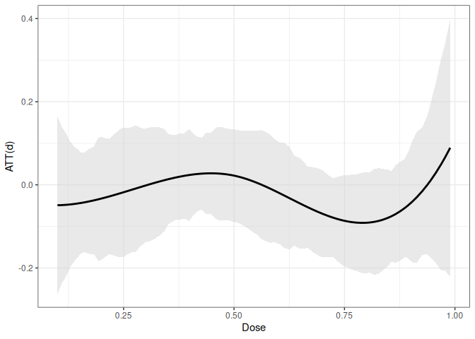
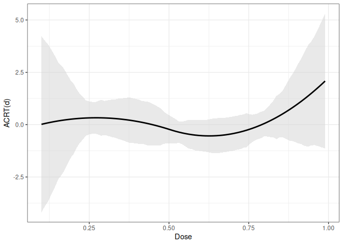
The following code can be used to estimate the ATT(d) and ACRT(d) parameters for the continuous treatment D using the cont_did function. The aggregation argument is set to “dose” and the target_parameter argument is set to “level” for ATT(d) and “slope” for ACRT(d).

cd_res <- cont_did(
  yname = "Y",
  tname = "time_period",
  idname = "id",
  dname = "D",
  data = df,
  gname = "G",
  target_parameter = "slope",
  aggregation = "dose",
  treatment_type = "continuous",
  control_group = "notyettreated",
  biters = 100,
  cband = TRUE,
  num_knots = 1,
  degree = 3,
)

summary(cd_res)
#> 
#> Overall ATT:  
#>      ATT    Std. Error     [ 95%  Conf. Int.] 
#>  -0.0265        0.0301    -0.0855      0.0325 
#> 
#> 
#> Overall ACRT:  
#>    ACRT    Std. Error     [ 95%  Conf. Int.]  
#>  0.1341        0.0485      0.039      0.2293 *
#> ---
#> Signif. codes: `*' confidence band does not cover 0
ggcont_did(cd_res, type = "att")

ggcont_did(cd_res, type = "acrt")

Case 2: Event Study Aggregations

Next, we consider event study aggregations. The first is an event study aggregation for ATT. The second is an event study aggregation for ACRT.

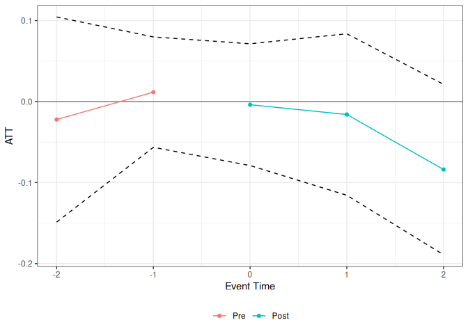
Event study aggregation for ATT:

Notice that the target parameter is set level to target ATT, and the aggregation argument is set to eventstudy.

cd_res_es_level <- cont_did(
  yname = "Y",
  tname = "time_period",
  idname = "id",
  dname = "D",
  data = df,
  gname = "G",
  target_parameter = "level",
  aggregation = "eventstudy",
  treatment_type = "continuous",
  control_group = "notyettreated",
  biters = 100,
  cband = TRUE,
  num_knots = 1,
  degree = 3,
)

summary(cd_res_es_level)
#> 
#> Overall ATT:  
#>      ATT    Std. Error     [ 95%  Conf. Int.] 
#>  -0.0243        0.0289    -0.0808      0.0323 
#> 
#> 
#> Dynamic Effects:
#>  Event Time Estimate Std. Error [95% Simult.  Conf. Band] 
#>          -2  -0.0222     0.0504       -0.1488      0.1044 
#>          -1   0.0116     0.0271       -0.0565      0.0798 
#>           0  -0.0039     0.0299       -0.0790      0.0713 
#>           1  -0.0160     0.0397       -0.1157      0.0837 
#>           2  -0.0839     0.0419       -0.1891      0.0212 
#> ---
#> Signif. codes: `*' confidence band does not cover 0
ggcont_did(cd_res_es_level)

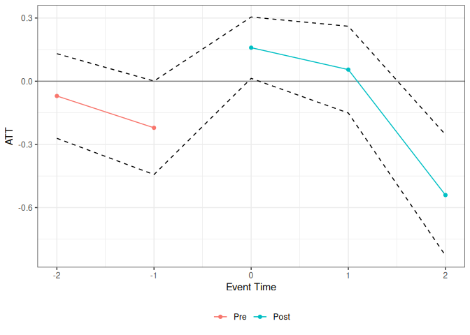
Event study aggregation for ACRT:

Relative to the previous code, notice that the target parameter is set slope to target ACRT.

cd_res_es_slope <- cont_did(
  yname = "Y",
  tname = "time_period",
  idname = "id",
  dname = "D",
  data = df,
  gname = "G",
  target_parameter = "slope",
  aggregation = "eventstudy",
  treatment_type = "continuous",
  control_group = "notyettreated",
  biters = 100,
  cband = TRUE,
  num_knots = 1,
  degree = 3,
)

summary(cd_res_es_slope)
#> 
#> Overall ACRT:  
#>     ATT    Std. Error     [ 95%  Conf. Int.]  
#>  0.1341        0.0584     0.0197      0.2485 *
#> 
#> 
#> Dynamic Effects:
#>  Event Time Estimate Std. Error [95% Simult.  Conf. Band]  
#>          -2  -0.0701     0.0808       -0.2710      0.1308  
#>          -1  -0.2212     0.0892       -0.4431      0.0007  
#>           0   0.1592     0.0586        0.0136      0.3048 *
#>           1   0.0551     0.0828       -0.1509      0.2610  
#>           2  -0.5405     0.1154       -0.8275     -0.2535 *
#> ---
#> Signif. codes: `*' confidence band does not cover 0
ggcont_did(cd_res_es_slope)

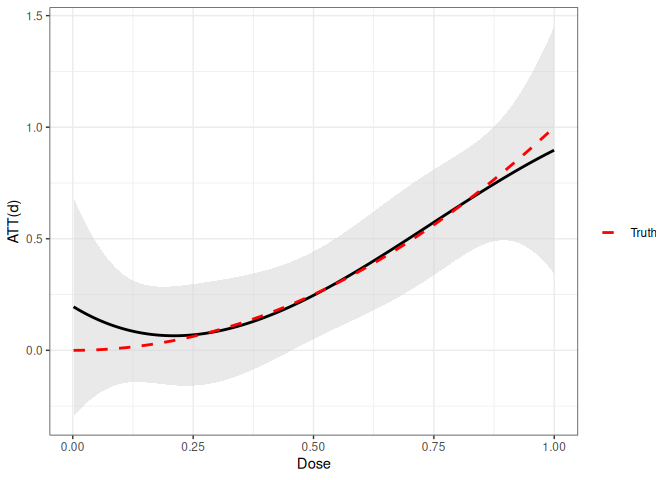
Case 3: Data-Driven Nonparametric Model for Treatment Effects

In most applications, it is hard to know the correct functional form for the treatment effects as a function of the dose. In Callaway et al. (2025), the approach we emphasize comes from Chen et al. (2025), and the contdid package uses their npiv package to implement this approach. Code-wise, the only thing to change is to set the argument dose_est_method="cck". [Note that we currently only support this option for the case with two periods and no staggered adoption. With more periods, you can average the pre- and post-treatment periods to reduce it to a two period case and then run the code below; in fact, this is what we did in the application in our paper.]

# simulate data with only two periods
# add quadratic effect to see how well we can detect it
# (note code will not "know" that the effect is quadratic)
df2 <- simulate_contdid_data(
  n = 5000,
  num_time_periods = 2,
  num_groups = 2,
  dose_linear_effect = 0,
  dose_quadratic_effect = 1
)
df2$D[df2$G == 0] <- 0
head(df2)
#>   id G        D time_period           Y
#> 1  1 2 0.890987           1  1.84272906
#> 2  1 2 0.890987           2  5.30890209
#> 3  2 0 0.000000           1  0.59423237
#> 4  2 0 0.000000           2  2.81443324
#> 5  3 0 0.000000           1  1.77438193
#> 6  3 0 0.000000           2 -0.01032246

cd_res_cck <- cont_did(
  yname = "Y",
  tname = "time_period",
  idname = "id",
  dname = "D",
  data = df2,
  gname = "G",
  target_parameter = "level",
  aggregation = "dose",
  treatment_type = "continuous",
  dose_est_method = "cck",
  control_group = "notyettreated",
  biters = 100,
  cband = TRUE,
)

summary(cd_res_cck)
#> 
#> Overall ATT:  
#>     ATT    Std. Error     [ 95%  Conf. Int.]  
#>  0.3399         0.037     0.2673      0.4125 *
#> 
#> 
#> Overall ACRT:  
#>    ACRT    Std. Error     [ 95%  Conf. Int.]  
#>  0.6595        0.1853     0.2964      1.0226 *
#> ---
#> Signif. codes: `*' confidence band does not cover 0
ggcont_did(cd_res_cck) +
  stat_function(
    fun = function(x) x^2,
    aes(color = "Truth"),
    linetype = "dashed",
    size = 1
  ) +
  scale_color_manual(values = c("Truth" = "red")) +
  labs(color = "")

References