Design of Experiments and Factorial Plans Utilities

A number of functions to create and analyze factorial plans according to the Design of Experiments (DoE) approach, with the addition of some utility function to perform some statistical analyses. DoE approach follows the approach in "Design and Analysis of Experiments" by Douglas C. Montgomery (2019, ISBN:978-1-119-49244-3). The package also provides utilities used in the course "Analysis of Data and Statistics" at the University of Trento, Italy.

adas.utils

The goal of adas.utils is to provide some utility functions to be used in the course Analysis of Data and Statistics at the University of Trento, Italy. Course contents are on https://paolobosetti.quarto.pub/ADAS/.

Installation

You can install the development version of adas.utils from GitHub with:

# install.packages("devtools")
devtools::install_github("pbosetti/adas.utils", build_vignettes = TRUE)

Examples

Loading data sets

On https://paolobosetti.quarto.pub/data.html there are a list of example datasets to be used during the course. You can load them with the examples_url function:

examples_url("battery.dat") |> read.table(header=T) |> head()
#>   RunOrder StandardOrder Temperature Material Repeat Response
#> 1       34             1          15        1      1      130
#> 2       25             2          70        1      1       34
#> 3       16             3         125        1      1       20
#> 4        7             4          15        2      1      150
#> 5        8             5          70        2      1      136
#> 6        1             6         125        2      1       25

Chauvenet’s criterion

The Chauvenet’s criterion is a method to identify possible outliers in a sample. Here is an example:

x <- rnorm(100)
x[50] <- 10
chauvenet(x)
#> Chauvenet's criterion for sample x
#> Suspect outlier: 50, value 10
#> Decision: reject it

Daniel’s plot

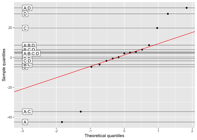
Daniel’s plot is a QQ plot of the effects of a non-replicated factorial model. Here is an example:

daniel_plot_qq(lm(Y~A*B*C*D, data=filtration))

### Tukey’s test plot

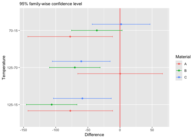
The stats::TukeyHSD function in base R provides a way to perform multiple comparisons of means. It can print the results in tabular form or can be plotted with the plot method:

library(tidyverse)
examples_url("battery.dat") %>%
  read_table() %>%
  mutate(across(c(Temperature, Material), factor)) %>%
  mutate(Material = LETTERS[Material]) %>% 
  ggTukey(Response~Temperature, splt=~Material)

Pareto chart

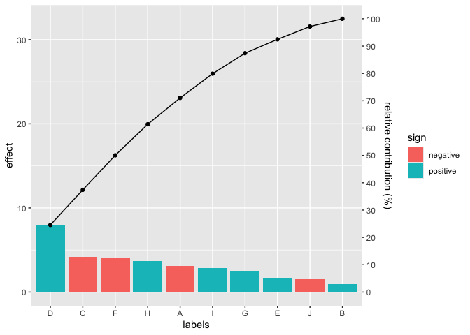
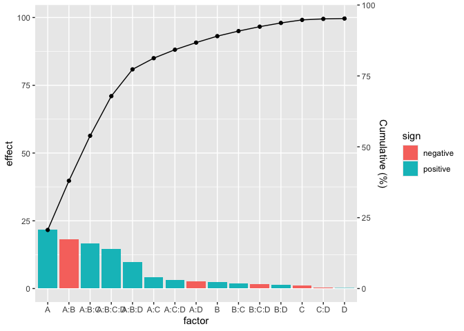
The pareto_chart function is a generic function that creates a Pareto chart either from a general data frame or from the effects of a lm object. Here is an example:

library(tidyverse)
set.seed(1)
tibble(
  val=rnorm(10, sd=5),
  cat=LETTERS[1:length(val)]
  ) %>%
  pareto_chart(labels=cat, values=val)
#> Warning in pareto_chart.data.frame(., labels = cat, values = val): 'pareto_chart.data.frame' is deprecated.
#> Use 'geom_pareto' instead.
#> See help("Deprecated")

# For a linear model:
pareto_chart(lm(Y~A*B*C*D, data=filtration))

Design of Experiments

There is a host of functions to be used in the context of Design of Experiments. Here is an example to prepare a design matrix for a $2^{5-2}$ fractional factorial plan:

fp_design_matrix(5) %>% 
  fp_fraction(~A*B*C*D) %>% 
  fp_fraction(~B*C*D*E)
#>  Factorial Plan Design Matrix
#>  Defining Relationship:  ~ A * B * C * D * E 
#>  Factors:  A B C D E 
#>  Levels:  -1 1 
#>  Fraction:  I=ABCD I=BCDE 
#>  Type:  fractional 
#>  
#> # A tibble: 8 × 12
#>   StdOrder RunOrder .treat  .rep     A     B     C     D     E Y      ABCD  BCDE
#>      <int>    <int> <chr>  <int> <dbl> <dbl> <dbl> <dbl> <dbl> <lgl> <dbl> <dbl>
#> 1        1        9 (1)        1    -1    -1    -1    -1    -1 NA        1     1
#> 2        7       14 bc         1    -1     1     1    -1    -1 NA        1     1
#> 3       11       10 bd         1    -1     1    -1     1    -1 NA        1     1
#> 4       13       31 cd         1    -1    -1     1     1    -1 NA        1     1
#> 5       20        4 abe        1     1     1    -1    -1     1 NA        1     1
#> 6       22       13 ace        1     1    -1     1    -1     1 NA        1     1
#> 7       26       26 ade        1     1    -1    -1     1     1 NA        1     1
#> 8       32       24 abcde      1     1     1     1     1     1 NA        1     1

You can also prepare a design matrix for a $2^n$ full factorial plan, and later on augment it with a central point and then to a central composite design with axial points:

fp_design_matrix(3, rep=2) %>% 
  fp_augment_center(rep=5) %>% 
  fp_augment_axial(rep=2)
#>  Factorial Plan Design Matrix
#>  Defining Relationship:  ~ A * B * C 
#>  Factors:  A B C 
#>  Levels:  -1 1 
#>  Fraction:  NA 
#>  Type:  composite 
#>  
#> # A tibble: 33 × 8
#>    StdOrder RunOrder .treat  .rep     A     B     C Y    
#>       <int>    <int> <chr>  <int> <dbl> <dbl> <dbl> <lgl>
#>  1        1       10 (1)        1    -1    -1    -1 NA   
#>  2        2        7 a          1     1    -1    -1 NA   
#>  3        3        3 b          1    -1     1    -1 NA   
#>  4        4       16 ab         1     1     1    -1 NA   
#>  5        5        6 c          1    -1    -1     1 NA   
#>  6        6        8 ac         1     1    -1     1 NA   
#>  7        7        2 bc         1    -1     1     1 NA   
#>  8        8       13 abc        1     1     1     1 NA   
#>  9        9       12 (1)        2    -1    -1    -1 NA   
#> 10       10       11 a          2     1    -1    -1 NA   
#> # ℹ 23 more rows

Author

Paolo Bosetti, University of Trento