Spatial Estimation and Prediction for Censored/Missing Responses

It provides functions for estimating parameters in linear spatial models with censored or missing responses using the Expectation-Maximization (EM), Stochastic Approximation EM (SAEM), and Monte Carlo EM (MCEM) algorithms. These methods are widely used to obtain maximum likelihood (ML) estimates in the presence of incomplete data. The EM algorithm computes ML estimates when a closed-form expression for the conditional expectation of the complete-data log-likelihood is available. The MCEM algorithm replaces this expectation with a Monte Carlo approximation based on independent simulations of the missing data. In contrast, the SAEM algorithm decomposes the E-step into simulation and stochastic approximation steps, improving computational efficiency in complex settings. In addition, the package provides standard error estimation based on the Louis method. It also includes functionality for spatial prediction at new locations. References used for this package: Galarza, C. E., Matos, L. A., Castro, L. M., & Lachos, V. H. (2022). Moments of the doubly truncated selection elliptical distributions with emphasis on the unified multivariate skew-t distribution. Journal of Multivariate Analysis, 189, 104944 ; Valeriano, K. A., Galarza, C. E., & Matos, L. A. (2023). Moments and random number generation for the truncated elliptical family of distributions. Statistics and Computing, 33(1), 32 .

The RcppCensSpatial package

The RcppCensSpatial package fits spatial censored linear regression models using the Expectation-Maximization (EM) (Dempster, Laird, and Rubin 1977), Stochastic Approximation EM (SAEM) (Delyon, Lavielle, and Moulines 1999), or Monte Carlo EM (MCEM) (Wei and Tanner 1990) algorithm. These algorithms are widely used to obtain maximum likelihood (ML) estimates in the presence of incomplete data. The EM algorithm can be applied when a closed-form expression for the conditional expectation of the complete-data log-likelihood is available. In the MCEM algorithm, this conditional expectation is replaced by a Monte Carlo approximation based on multiple independent simulations of the partially observed data. In contrast, the SAEM algorithm decomposes the E-step into simulation and stochastic approximation steps.

The package also provides approximate standard errors for the parameter estimates using the method proposed by Louis (1982), and it supports missing values in the response variable. In addition, it includes functions for spatial prediction at new locations, as well as for computing covariance and distance matrices. For further details on model formulation and estimation procedures, see Ordoñez et al. (2018) and Valeriano et al. (2021).

The RcppCensSpatial library provides the following functions:

• CovMat: computes the spatial covariance matrix.
• dist2Dmatrix: computes the Euclidean distance matrix for a set of coordinates.
• EM.sclm: fits a spatial censored linear regression model using the EM algorithm.
• MCEM.sclm: fits a spatial censored linear regression model using the MCEM algorithm.
• SAEM.sclm: fits a spatial censored linear regression model using the SAEM algorithm.
• predict.sclm: performs spatial prediction at a set of new locations.
• rCensSp: simulates censored spatial data under a specified censoring rate.

The generic functions print, summary, predict, and plot are also available for objects of class sclm.

In the following sections, we describe how to install the package and demonstrate the use of its main functions through an artificial example.

Installation

The released version of RcppCensSpatial from CRAN can be installed with:

install.packages("RcppCensSpatial")

Example

In the following example, we simulate a dataset of size n = 220 from a spatial linear regression model with three covariates and an exponential correlation function to account for spatial dependence. To evaluate predictive performance, the dataset is split into training and testing sets. The training set consists of 200 observations, with 5% left-censored responses, while the test set contains the remaining 20 observations.

library(RcppCensSpatial)

set.seed(12341)
n = 220
x = cbind(1, runif(n), rnorm(n))
coords = round(matrix(runif(2*n, 0, 15), n, 2), 5)
dat = rCensSp(beta=c(1,2,-1), sigma2=1, phi=4, nugget=0.50, x=x, coords=coords,
              cens='left', pcens=.05, npred=20, cov.model="exponential")
# Proportion of censoring
table(dat$Data$ci)
#> 
#>   0   1 
#> 190  10

For comparison purposes, we fit the spatial censored linear model to the simulated data using three approaches: the EM, MCEM, and SAEM algorithms. Each method is run with the same maximum number of iterations (MaxIter = 300) and uses the exponential spatial correlation function (type = "exponential"), which is also the default setting and was used in the data generation process.

Other available spatial correlation functions include 'matern', 'gaussian', and 'pow.exp'.

data1 = dat$Data

# EM estimation
fit1 = EM.sclm(data1$y, data1$x, data1$ci, data1$lcl, data1$ucl, data1$coords, 
               phi0=3, nugget0=1, MaxIter=300)
fit1$tab
#>       beta0  beta1   beta2 sigma2    phi   tau2
#>      0.6959 1.7894 -0.9477 1.2032 4.3018 0.3824
#> s.e. 0.4848 0.2027  0.0592 0.5044 2.2872 0.0793

# MCEM estimation
fit2 = MCEM.sclm(data1$y, data1$x, data1$ci, data1$lcl, data1$ucl, data1$coords, 
                 phi0=3, nugget0=1, MaxIter=300, nMax=1000)
fit2$tab
#>       beta0  beta1   beta2 sigma2    phi   tau2
#>      0.6952 1.7896 -0.9476 1.2069 4.3216 0.3828
#> s.e. 0.4868 0.2025  0.0592 0.5121 2.3144 0.0793

# SAEM estimation
fit3 = SAEM.sclm(data1$y, data1$x, data1$ci, data1$lcl, data1$ucl, data1$coords, 
                 phi0=3, nugget0=1, M=10)
fit3$tab
#>       beta0  beta1   beta2 sigma2    phi   tau2
#>      0.6959 1.7883 -0.9471 1.2060 4.3207 0.3811
#> s.e. 0.4865 0.2021  0.0590 0.5096 2.3125 0.0791

Note that the parameter estimates obtained from each method are similar and generally close to the true values, except for the first regression coefficient, which is estimated to be approximately 0.70, whereas its true value is 1.

Moreover, the generic functions print and summary provide detailed information about the fitted sclm object, including parameter estimates, standard errors, the effective range, information criteria, and convergence diagnostics.

print(fit3)
#> ----------------------------------------------------------------
#>            Spatial Censored Linear Regression Model   
#> ----------------------------------------------------------------
#> Call:
#> SAEM.sclm(y = data1$y, x = data1$x, ci = data1$ci, lcl = data1$lcl, 
#>     ucl = data1$ucl, coords = data1$coords, phi0 = 3, nugget0 = 1, 
#>     M = 10)
#> 
#> Estimated parameters:
#>       beta0  beta1   beta2 sigma2    phi   tau2
#>      0.6959 1.7883 -0.9471 1.2060 4.3207 0.3811
#> s.e. 0.4865 0.2021  0.0590 0.5096 2.3125 0.0791
#> 
#> The effective range is 12.9436 units.
#> 
#> Model selection criteria:
#>         Loglik     AIC     BIC
#> Value -251.323 514.645 534.435
#> 
#> Details:
#> Number of censored/missing values: 10 
#> Convergence reached?: TRUE 
#> Iterations: 161 / 300 
#> Processing time: 1.0391 mins

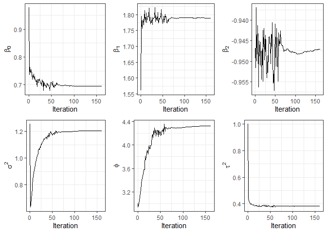
Additionally, the plot function can be used to visualize convergence diagnostics of the parameter estimates.

plot(fit3)

Next, predicted values are obtained for each fitted model on the test data, and their mean squared prediction errors (MSPE) are compared.

data2 = dat$TestData
pred1 = predict(fit1, data2$coords, data2$x)
pred2 = predict(fit2, data2$coords, data2$x)
pred3 = predict(fit3, data2$coords, data2$x)

# Cross-validation
mean((data2$y - pred1$predValues)^2)
#> [1] 1.595305
mean((data2$y - pred2$predValues)^2)
#> [1] 1.591421
mean((data2$y - pred3$predValues)^2)
#> [1] 1.594899

References

Delyon, B., M. Lavielle, and E. Moulines. 1999. “Convergence of a Stochastic Approximation Version of the EM Algorithm.” The Annals of Statistics 27 (1): 94–128.
Dempster, A. P., N. M. Laird, and D. B. Rubin. 1977. “Maximum Likelihood from Incomplete Data via the EM Algorithm.” Journal of the Royal Statistical Society: Series B (Methodological) 39 (1): 1–38.
Louis, T. A. 1982. “Finding the Observed Information Matrix When Using the EM Algorithm.” Journal of the Royal Statistical Society: Series B (Methodological) 44 (2): 226–33.
Ordoñez, J. A., D. Bandyopadhyay, V. H. Lachos, and C. R. B. Cabral. 2018. “Geostatistical Estimation and Prediction for Censored Responses.” Spatial Statistics 23: 109–23. https://doi.org/10.1016/j.spasta.2017.12.001.
Valeriano, K. L., V. H. Lachos, M. O. Prates, and L. A. Matos. 2021. “Likelihood-Based Inference for Spatiotemporal Data with Censored and Missing Responses.” Environmetrics 32 (3).
Wei, G., and M. Tanner. 1990. “A Monte Carlo Implementation of the EM Algorithm and the Poor Man’s Data Augmentation Algorithms.” Journal of the American Statistical Association 85 (411): 699–704. https://doi.org/10.1080/01621459.1990.10474930.