Multi-Armed Bandit Approaches to Pricing Experiments

Implements multi-armed bandit approaches for pricing experiments with an unknown demand curve, as developed in Weaver, Kumar, and Jain (2025) "Nonparametric Pricing Bandits Leveraging Informational Externalities to Learn the Demand Curve" . Includes Upper Confidence Bound (UCB) and Thompson Sampling (TS) baselines, Gaussian process variants (GP-UCB, GP-TS), monotonic Gaussian process variants that constrain demand to be weakly decreasing in price, and heterogeneous-noise extensions. The willingness-to-pay distribution is fully user-specified via a vector of consumer valuations, so any demand environment can be simulated or replayed.

PricingBandits

Multi-armed bandit approaches to pricing experiments with an unknown demand curve, from:

Weaver, I. N., Kumar, V., & Jain, L. Nonparametric Pricing Bandits Leveraging Informational Externalities to Learn the Demand Curve. Marketing Science.

This package contains the streamlined, core bandit machinery. The full replication code for the paper (WTP construction, expected-reward analysis, figures) lives in the separate replication repository; results from this package are validated seed-for-seed bit-identical against it.

Looking for the Python version? See pricingbandits-py.

Installation

# from CRAN (released version):
install.packages("PricingBandits")

# or the development version from GitHub:
# install.packages("devtools")
devtools::install_github("ian-weaver/PricingBandits")

Quick start

You supply one consumer valuation (willingness to pay) per round — drawn from any distribution you like — plus a set of candidate prices. The chosen policy prices each arriving consumer and learns from buy/no-buy feedback alone.

library(PricingBandits)

set.seed(1)
valuations <- rbeta(2500, 2, 9)          # any WTP process you like

out <- PricingBandit(valuations,
                     prices     = seq(10)/10,
                     policy     = "GP-TS-M",
                     batch_size = 10)

table(out$PricesTested)
attr(out, "diagnostics")

Policies

Options: hetero = TRUE enables the heterogeneous-noise extension for GP variants; reset = n wipes the history every n consumers (time-varying demand); num_knots controls the monotonic variants' constraint grid and defaults to 11 regardless of the number of arms — with many more knots the truncated sampler operates in a near-degenerate high-dimensional space and can break down, so keep it modest even for dense price grids. timeout (default 5 seconds) bounds each truncated-sampling attempt before the fallback chain advances; raise it on slow machines, lower it to fail over to cheaper approximations sooner.

Policy Comparison Example

Running each policy with one seed on the same 1,000 consumers — willingness to pay drawn from a Beta(2, 9) distribution — gives the results below. To compare policies, score each price the bandit posted by its expected revenue under the true distribution, and track the cumulative total as a percentage of what always charging the optimal price would have earned:

expected_revenue <- prices * (1 - pbeta(prices, 2, 9))   # true revenue at each posted price
grid             <- seq(1e-6, 1, 1e-6)
optimal          <- max(grid * (1 - pbeta(grid, 2, 9)))  # best any price could do
earned           <- expected_revenue[match(out$PricesTested, prices)]
pct_of_optimal   <- cumsum(earned) / (seq_along(earned) * optimal) * 100

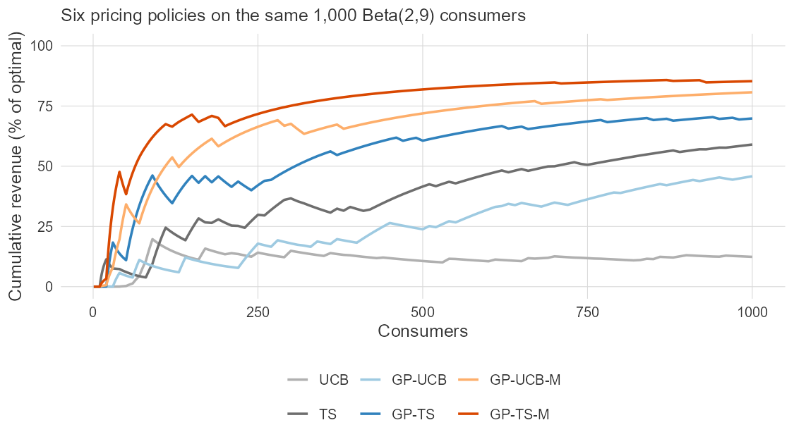
See the package vignette for the full walk-through this figure comes from, including the heterogeneous-noise variants and every argument explained.

Diagnostics

Every run counts the numerical fallback paths (hyperparameter-optimization failures, truncated-sampler timeouts, last-resort samplers); in normal operation these are all zero. See GetDiagnostics().