Nonlinear Vector Autoregression Models

Estimate nonlinear vector autoregression models (also known as the next generation reservoir computing) for nonlinear dynamic systems. The algorithm was described by Gauthier et al. (2021) .

NVAR: Nonlinear Vector Autoregression Models

Estimate nonlinear vector autoregression models (also known as the next generation reservoir computing) for nonlinear dynamic systems. The algorithm was described by Gauthier et al. (2021) doi:10.1038/s41467-021-25801-2.

Installation

You can install the development version of NVAR from GitHub with:

# install.packages("devtools")
devtools::install_github("Sciurus365/NVAR")

Example

This is an example for the Lorenz model.

library(NVAR)

testdata <- nonlinearTseries::lorenz()
testdata <- tibble::as_tibble(testdata)
t1 <- NVAR(data = testdata, vars = c("x", "y", "z"), s = 2, k = 2, p = 2, alpha = 1e-3)
t1_sim <- sim_NVAR(t1, length = 5000)


realdata <- nonlinearTseries::lorenz(time = seq(0, 100, by = .01)) %>% tibble::as_tibble()

library(ggplot2)
ggplot(realdata) +
  geom_line(aes(x = 1:10001, y = x), color = "red", alpha = 0.4) +
  geom_line(aes(x = 1:10001, y = x), data = t1_sim, color = "blue", alpha = 0.4) +
  geom_vline(xintercept = 5000) +
  theme_bw() +
  xlim(c(4900, 8000)) +
  labs(x = "time", y = "x")

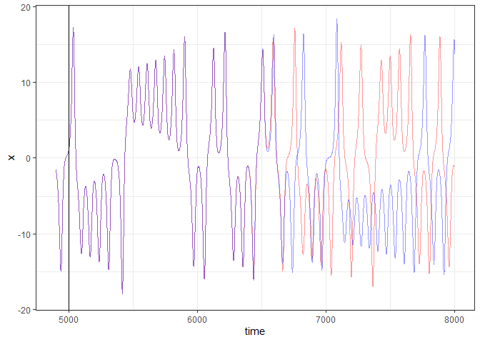
# Red line: real data.
# Blue line: simulated data with the NVAR.
# Black vertical line: when the simulation starts.