LDATree
Oblique Classification Trees with Uncorrelated Linear Discriminant Analysis Splits
A classification tree method that uses Uncorrelated Linear Discriminant Analysis (ULDA) for variable selection, split determination, and model fitting in terminal nodes. It automatically handles missing values and offers visualization tools. For more details, see Wang (2024)
LDATree 

LDATree is an R modeling package for fitting classification trees with
oblique splits.
-
If you are unfamiliar with classification trees, here is a tutorial about the traditional CART and its R implementation
rpart. -
More details about the LDATree can be found in Wang, S. (2024). FoLDTree: A ULDA-Based Decision Tree Framework for Efficient Oblique Splits and Feature Selection. arXiv preprint arXiv:2410.23147. Link.
Overview
Compared to other similar trees, LDATree distinguishes itself in the
following ways:
-
Using Uncorrelated Linear Discriminant Analysis (ULDA) from the
foldapackage, it can efficiently find oblique splits. -
It provides both ULDA and forward ULDA as the splitting rule and node model. Forward ULDA has intrinsic variable selection, which helps mitigate the influence of noise variables.
-
It automatically handles missing values.
-
It can output both predicted class and class probability.
-
It supports downsampling, which can be used to balance classes or accelerate the model fitting process.
-
It includes several visualization tools to provide deeper insights into the data.
Installation
install.packages("LDATree")
You can install the development version of LDATree from
GitHub with:
# install.packages("devtools")
devtools::install_github('Moran79/LDATree')
Basic Usage
We offer two main tree types in the LDATree package: LDATree and
FoLDTree. For the splitting rule and node model, LDATree uses ULDA,
while FoLDTree uses forward ULDA.
To build an LDATree (or FoLDTree):
library(LDATree)
set.seed(443)
diamonds <- as.data.frame(ggplot2::diamonds)[sample(53940, 2000),]
datX <- diamonds[, -2]
response <- diamonds[, 2] # we try to predict "cut"
fit <- Treee(datX = datX, response = response, verbose = FALSE) # by default, it is a pre-stopping FoLDTree
# fit <- Treee(datX = datX, response = response, verbose = FALSE, ldaType = "all", pruneMethod = "post") # if you want to fit a post-pruned LDATree.
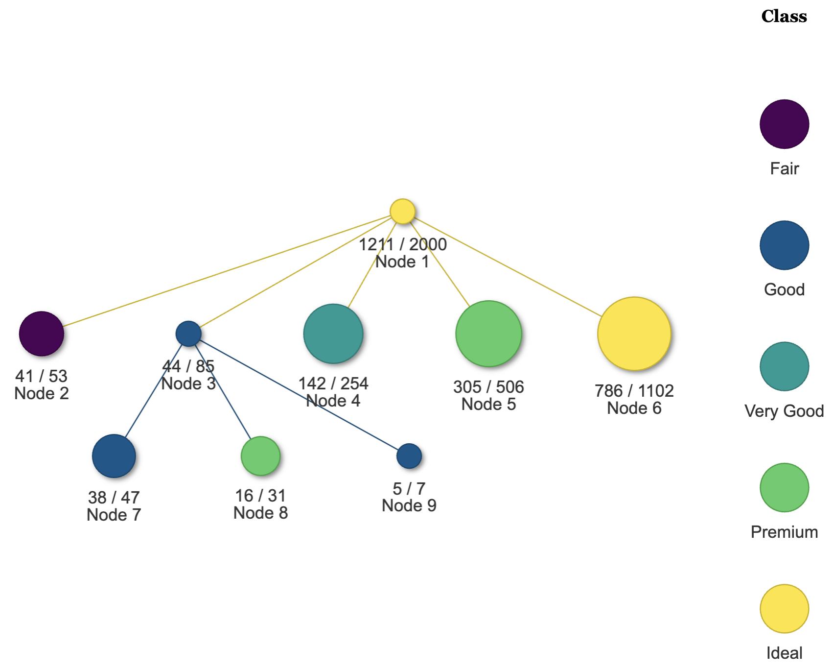
To plot the LDATree (or FoLDTree):
# View the overall tree.
plot(fit)
# Three types of individual plots
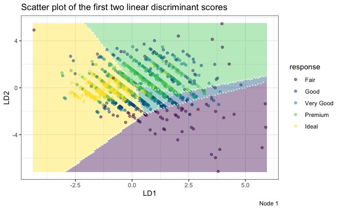
# 1. Scatter plot on first two LD scores
plot(fit, datX = datX, response = response, node = 1)
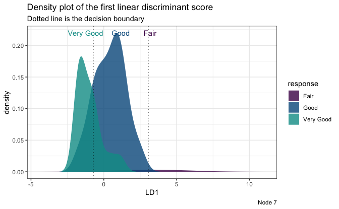
# 2. Density plot on the first LD score
plot(fit, datX = datX, response = response, node = 7)
# 3. A message
plot(fit, datX = datX, response = response, node = 2)
#> [1] "Every observation in node 2 is predicted to be Fair"
To make predictions:
# Prediction only.
predictions <- predict(fit, datX)
head(predictions)
#> [1] "Ideal" "Ideal" "Ideal" "Ideal" "Ideal" "Ideal"
# A more informative prediction
predictions <- predict(fit, datX, type = "all")
head(predictions)
#>   response node         Fair        Good Very Good     Premium     Ideal
#> 1    Ideal    6 4.362048e-03 0.062196349 0.2601145 0.056664046 0.6166630
#> 2    Ideal    6 1.082022e-04 0.006308281 0.1290079 0.079961227 0.7846144
#> 3    Ideal    6 7.226446e-03 0.077434549 0.2036148 0.023888946 0.6878352
#> 4    Ideal    6 1.695119e-02 0.115233616 0.1551836 0.008302145 0.7043295
#> 5    Ideal    6 4.923729e-05 0.004157352 0.1498265 0.187391975 0.6585749
#> 6    Ideal    6 4.827312e-03 0.061274797 0.1978061 0.027410359 0.7086815
More examples can be found in the vignette.
References
- Wang, S. (2024). FoLDTree: A ULDA-based decision tree framework for efficient oblique splits and feature selection. arXiv preprint, arXiv:2410.23147. Retrieved from https://arxiv.org/abs/2410.23147.
Getting help
If you encounter a clear bug, please file an issue with a minimal reproducible example on GitHub