Analytic Element Modeling of Steady Single-Layer Groundwater Flow

A model of single-layer groundwater flow in steady-state under the Dupuit-Forchheimer assumption can be created by placing elements such as wells, area-sinks and line-sinks at arbitrary locations in the flow field. Output variables include hydraulic head and the discharge vector. Particle traces can be computed numerically in three dimensions. The underlying theory is described in Haitjema (1995) and references therein.

raem

raem is an R package for modeling steady-state, single-layer groundwater flow under the Dupuit-Forchheimer assumption using analytic elements.

Installation

To install the released version:

install.packages("raem")

The development version of raem can be installed from GitHub with:

# install.packages("devtools")
devtools::install_github("cneyens/raem")

Documentation

The package documentation can be found at https://cneyens.github.io/raem/.

Example

Construct an analytic element model of an aquifer with uniform background flow, two extraction wells and a reference point.

Specify the aquifer parameters and create the elements:

library(raem)

# aquifer parameters ----
k = 10     # hydraulic conductivity, m/d
top = 10   # aquifer top elevation, m
base = 0   # aquifer bottom elevation, m
n = 0.2    # aquifer porosity, -

hr = 15    # head at reference point, m
TR = k * (top - base) # constant transmissivity of background flow, m^2/d

# create elements ----
uf = uniformflow(TR, gradient = 0.001, angle = -45)
rf = constant(xc = -1000, yc = 0, hc = hr)
w1 = well(xw = 200, yw = 0, Q = 250)
w2 = well(xw = -200, yw = -150, Q = 400)

Create the model. This automatically solves the system of equations.

m = aem(k = k, top = top, base = base, n = n, uf, rf, w1, w2)

Find the head and discharge at two locations: x = -200, y = 200 and x = 100, y = 200. Note that there are no vertical flow components in this model:

heads(m, x = c(-200, 100), y = 200)
#> [1] 13.64573 13.33314

discharge(m, c(-200, 100), 200, z = top) # m^2/d
#>              Qx         Qy Qz
#> [1,] 0.15028815 -0.2923908  0
#> [2,] 0.06041242 -0.3347206  0

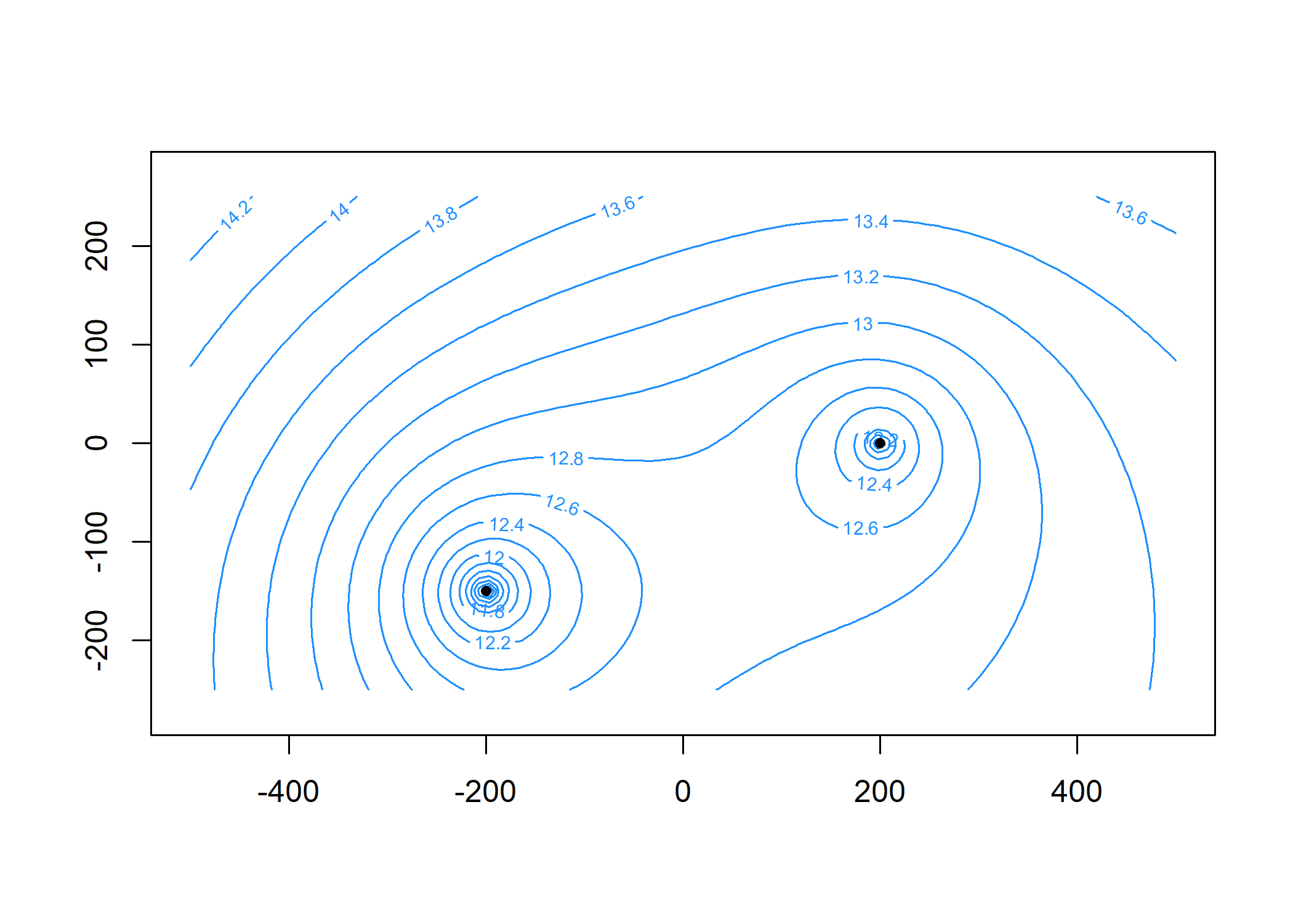
Plot the head contours and element locations. First, specify the contouring grid:

xg = seq(-500, 500, length = 100)
yg = seq(-250, 250, length = 100)

Now plot:

contours(m, xg, yg, 'heads', col = 'dodgerblue', nlevels = 20)
plot(m, add = TRUE)

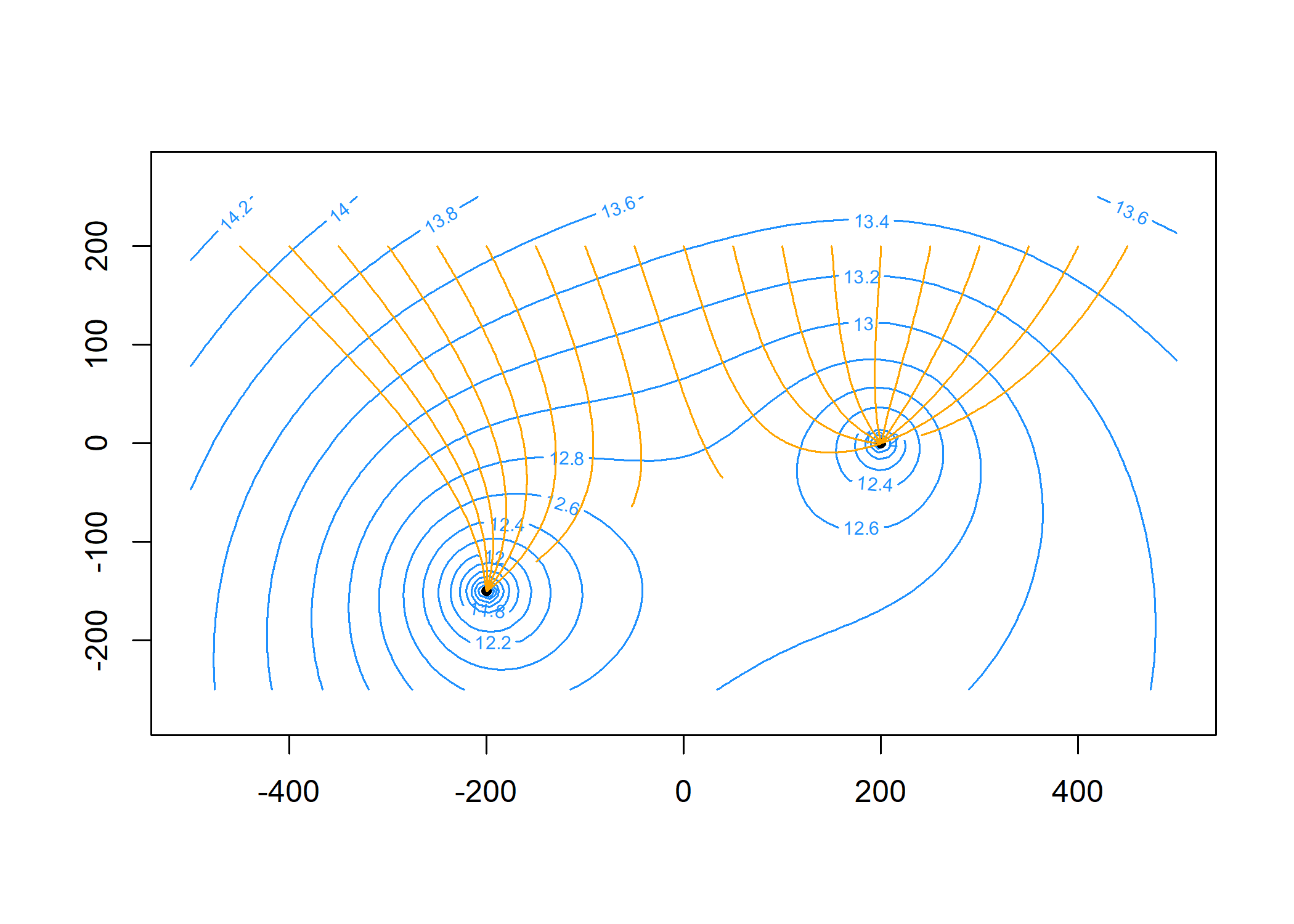
Compute particle traces starting along y = 200 at 20 intervals per year for 5 years and add to the plot:

paths = tracelines(m, 
                   x0 = seq(-450, 450, 50), 
                   y0 = 200, 
                   z0 = top, 
                   times = seq(0, 5 * 365, 365 / 20))

plot(paths, add = TRUE, col = 'orange')