Geometric Methods for Nonparametric Regression and Density Estimation

Provides geometric methods for nonparametric regression and density estimation on data represented as coordinate matrices or weighted graphs. Methods include local polynomial smoothing, model-averaged local polynomial smoothing, local polynomial lifting trend filtering, synchronized local polynomial lifting trend filtering, order-2 Gaussian and logistic trend filtering, graph low-pass filtering, and Hessian-energy regression. Methodological references include Gajer and Ravel (2025) "Adaptive Geometric Regression for High-Dimensional Structured Data" , Fan and Gijbels (1996, ISBN:9780412983214), Wang et al. (2016) "Trend Filtering on Graphs" < https://www.jmlr.org/papers/v17/15-147.html>, and Kim et al. (2009) "Semi-Supervised Regression Using Hessian Energy" < https://papers.nips.cc/paper/3741-semi-supervised-regression-using-hessian-energy-with-an-application-to-semi-supervised-dimensionality-reduction>.

geosmooth

geosmooth is an R package for nonparametric regression and density estimation when the data have geometric structure. The data can be given as a matrix of coordinates, one row per observation, or as a weighted graph whose vertices are the observations. The package estimates a smooth response, or a probability mass, over those points. Its methods include local polynomial smoothing, model-averaged local polynomial smoothing, two forms of local polynomial lifting trend filtering, one-dimensional Gaussian and logistic trend filtering, graph low-pass filtering, and Hessian-energy regression.

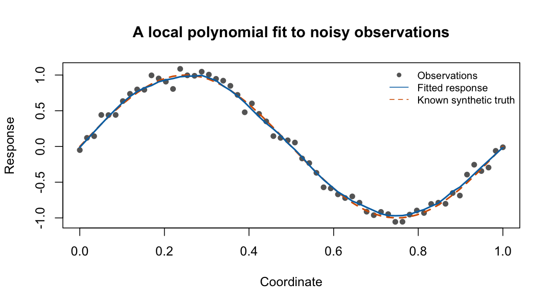
In the figure, the points are noisy observations, the solid line is a local polynomial fit whose settings were selected by cross-validation, and the dashed line is the true curve, which is known here because the data are simulated. The first-fit guide gives the code, the selected settings, and an explanation of the tuning score.

Where to start

• Finding your way around geosmooth is organized by task. It lists every exported function, says which fitted models can predict at new points, and includes examples. In an installed package, open it with vignette("function-guide", package = "geosmooth").
• help("geosmooth-package", package = "geosmooth") is a shorter overview with links to the main functions.
• The online reference is available by task and alphabetically.
• The synthetic datasets guide shows how to generate reproducible test data.
• NEWS describes what changed between versions and how to update existing code.

Installation

Install the released version from CRAN:

install.packages("geosmooth")
help("geosmooth-package", package = "geosmooth")

To install the development version from GitHub, you need the tools for compiling R packages from source:

install.packages("pak")
pak::pkg_install("pgajer/geosmooth")
vignette("function-guide", package = "geosmooth")

Version 0.2.0 requires R >= 4.1.0 and dgraphs >= 0.4.0. The optional GRIP and edge-KK embeddings also require grip >= 0.3.0.

Quick Start

library(geosmooth)

set.seed(1)
x <- seq(0, 1, length.out = 60)
X <- cbind(x = x)
y <- sin(2 * pi * x) + rnorm(length(x), sd = 0.08)
foldid <- rep(1:5, length.out = length(y))

lps.fit <- fit.lps(
    X = X,
    y = y,
    foldid = foldid,
    support.grid = c(8L, 12L, 16L),
    degree.grid = 0:1,
    kernel.grid = "gaussian"
)

head(predict(lps.fit))

fit.lps() fits a local polynomial smoother (LPS). It selects the neighborhood size, the degree of the local polynomial, and the kernel by cross-validation.

Choosing a method

The methods differ in the kind of data they take and in how they penalize roughness. The main ones are listed here; the function guide covers the rest.

• Local polynomial smoothing (LPS), fit.lps(). Fits a weighted polynomial to the observations near each point at which a prediction is wanted. This is the standard local-regression method and a good first choice.

• Model-averaged local polynomial smoothing (MALPS), fit.malps(). Fits a local polynomial around each of a set of anchor points and predicts at a point by averaging the local fits that cover it.

• Local polynomial lifting trend filtering (LPL-TF), fit.lpl.tf() and lpl.tf.operator(). Penalizes the absolute values of the residuals that remain when each fitted value is predicted from its neighbors by a local polynomial. As in trend filtering, this L1 penalty lets the fit adapt to the local smoothness of the response.

• Synchronized LPL-TF (S-LPL-TF, also called SLPLiFT), fit.slpl.tf() and slpl.tf.operator(). Adds to LPL-TF a quadratic penalty that makes the local predictions agree where their neighborhoods overlap.

• Graph low-pass filtering, fit.metric.graph.lowpass(). Smooths a response defined on the vertices of an undirected graph whose edges carry positive lengths or nonnegative conductances. The graph workflow explains how responses are matched to vertices, how lengths are converted to conductances, and how to reuse the computed eigenvectors for further responses. The observed-data heat guide covers missing responses and the numerical checks that are available.

• One-dimensional Gaussian trend filtering, fit.gaussian.trend.filtering(). Fits a piecewise-quadratic curve (trend filtering of order 2) to a continuous outcome. Its companion, assess.gaussian.trend.filtering(), tests by permutation whether the outcome varies with the predictor, repeating the tuning for every permutation, and compares held-out prediction error with that of a constant mean. The permutation test assumes that the outcomes are exchangeable under the null hypothesis; a constant mean with unequal variances is not enough.

• One-dimensional logistic trend filtering, fit.logistic.trend.filtering(). Fits the probability of a binary outcome as a function of a continuous predictor. assess.logistic.trend.filtering() tests by permutation whether the probability is constant and measures the gain in held-out prediction. The logistic trend-filtering guide works through simulated data and the Pima diabetes data.

• Hessian-energy regression, fit.ssrhe.hessian.regression() and fit.ssrhe.hessian.l1.regression(). Penalizes estimated second derivatives of the fit on a point cloud, following the semi-supervised regression with Hessian energy (SSRHE) of Kim, Steinke, and Hein (2009). The first function uses a quadratic penalty and the second an L1 penalty. Neighborhoods can have a fixed number of points, be supplied by you, or have radii that adapt to a graph.

Basic examples

The examples below continue from the Quick Start and use its X, y, and foldid.

LPS

lps.fit <- fit.lps(
    X = X,
    y = y,
    foldid = foldid,
    support.grid = c(8L, 12L),
    degree.grid = 0:1,
    kernel.grid = "gaussian"
)

lps.pred <- predict(lps.fit, X)

MALPS

malps.fit <- fit.malps(
    X = X,
    y = y,
    degree = 1L,
    support.type = "knn",
    support.size = 12L,
    kernel = "tricube",
    support.selection = "fixed",
    coordinate.method = "coordinates"
)

LPL-TF and S-LPL-TF

The operators can be built once and reused for several responses.

lpl.op <- lpl.tf.operator(
    X = X,
    degree = 1L,
    support.type = "knn",
    support.size = 12L,
    kernel = "gaussian",
    coordinate.method = "coordinates"
)

slpl.op <- slpl.tf.operator(
    X = X,
    degree = 1L,
    support.type = "knn",
    support.size = 12L,
    kernel = "gaussian",
    coordinate.method = "coordinates"
)

Fitting these two models requires the optional package genlasso.

if (requireNamespace("genlasso", quietly = TRUE)) {
    lpl.fit <- fit.lpl.tf(
        y = y,
        operator = lpl.op,
        lambda = 0.1,
        lambda.selection = "fixed"
    )

    slpl.fit <- fit.slpl.tf(
        y = y,
        operator = slpl.op,
        lambda1 = 0.1,
        lambda2 = 0.01,
        lambda.selection = "fixed"
    )
}

Hessian-energy regression

grid <- expand.grid(x = seq(0, 1, length.out = 5),
                    y = seq(0, 1, length.out = 5))
X2 <- as.matrix(grid)
y2 <- sin(2 * pi * X2[, 1]) + 0.25 * X2[, 2]

ssrhe.fit <- fit.ssrhe.hessian.regression(
    X = X2,
    y = y2,
    k = 12L,
    tangent.dim = 2L,
    lambda1 = 0.05,
    return.local.diagnostics = FALSE
)

# The same function can select the penalties by cross-validation
# (or by "gcv" when every response is observed).
ssrhe.cv <- fit.ssrhe.hessian.regression(
    X = X2,
    y = y2,
    k = 12L,
    tangent.dim = 2L,
    lambda.selection = "cv",
    lambda1.grid = c(0.01, 0.05, 0.2),
    cv.control = list(cv.folds = 5L)
)

The code of these examples is also available in inst/examples/geosmooth_quickstart.R.

Graphs and the dgraphs package

geosmooth does not construct graphs. Methods that work directly on coordinates need no graph: LPS, MALPS, and both lifting trend filters with coordinate neighborhoods, and Hessian-energy regression with neighborhoods of fixed size or neighborhoods that you supply. Methods that use distances along a graph take a graph object from the dgraphs package, which also computes the shortest paths. These are MALPS and the lifting trend filters with graph-geodesic neighborhoods, and Hessian-energy regression with adaptive-radius neighborhoods.

Compiled code

The computationally demanding parts of the package are written in C++: LPS cross-validation and prediction, the construction of local PCA coordinate charts, graph low-pass filtering, and the Hessian-energy operators.

Development

To run the main tests and a quick package check from a source checkout:

make test
make check-fast